Technical Goals
Smooth corners are a fundamental rendering primitive in a system UI. They appear in buttons, cards, masks, icon containers, panel corners, and many other places, with radii potentially ranging from to .
The technical solution therefore needs to meet four requirements at once:
- Stable shapes, without noticeable distortion when scaled
- Smooth edges, without visible jaggedness in high-contrast conditions
- Manageable runtime cost, without repeating expensive calculations for every corner in the system
- Broad applicability, supporting long-term evolution from 2D UI to more complex real-time rendering scenarios
Technical Architecture

The pipeline can be summarized in four steps:
- Define the ideal corner shape using a curve with high-order continuity.
- Rasterize the vector curve into a cached texture using high-quality anti-aliasing.
- Generate multiple mipmap levels from the cached image for stable rendering at different scales.
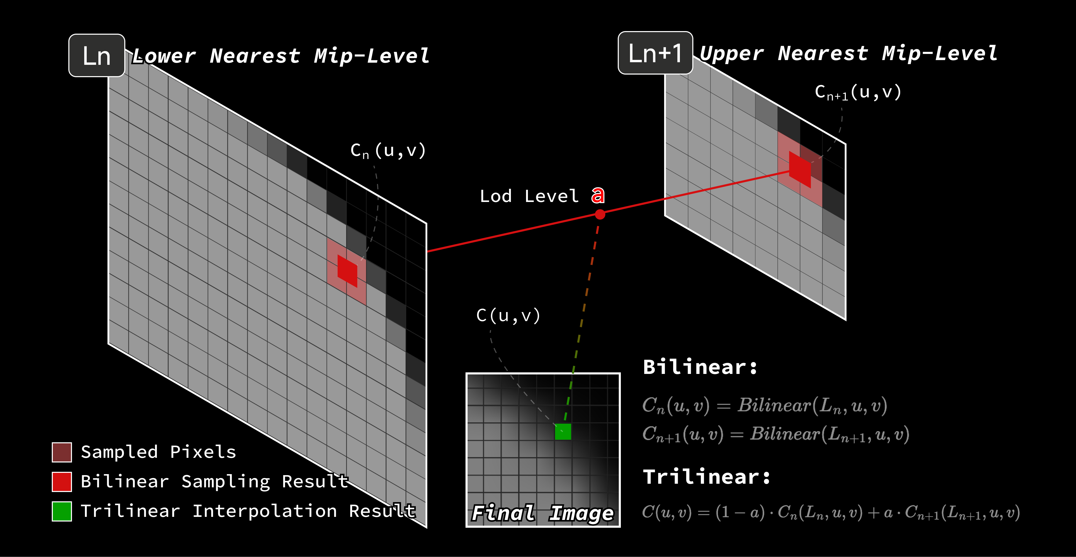
- Filter and sample the texture on the GPU at the appropriate level of detail (LOD), then output it to the screen.
The key is to move as much expensive, high-quality work as possible into offline processing or precomputation, leaving runtime work to the sampling operations GPUs handle best.
Curve Modeling: Why Degree-4 NURBS?
NURBS (non-uniform rational B-spline) curves offer a high degree of control, including fairly direct control over local curvature changes. In this project, curve modeling needed to satisfy two requirements:
- Achieve G4 geometric continuity: the corner is both a visual element and a geometric foundation that may feed into lighting, normal generation, and other rendering stages. Higher continuity leaves more room for future uses.
- Stay as close as possible to a circular arc: many existing system elements are already visually associated with circular corners, so an upgrade should not abruptly change the platform's character.
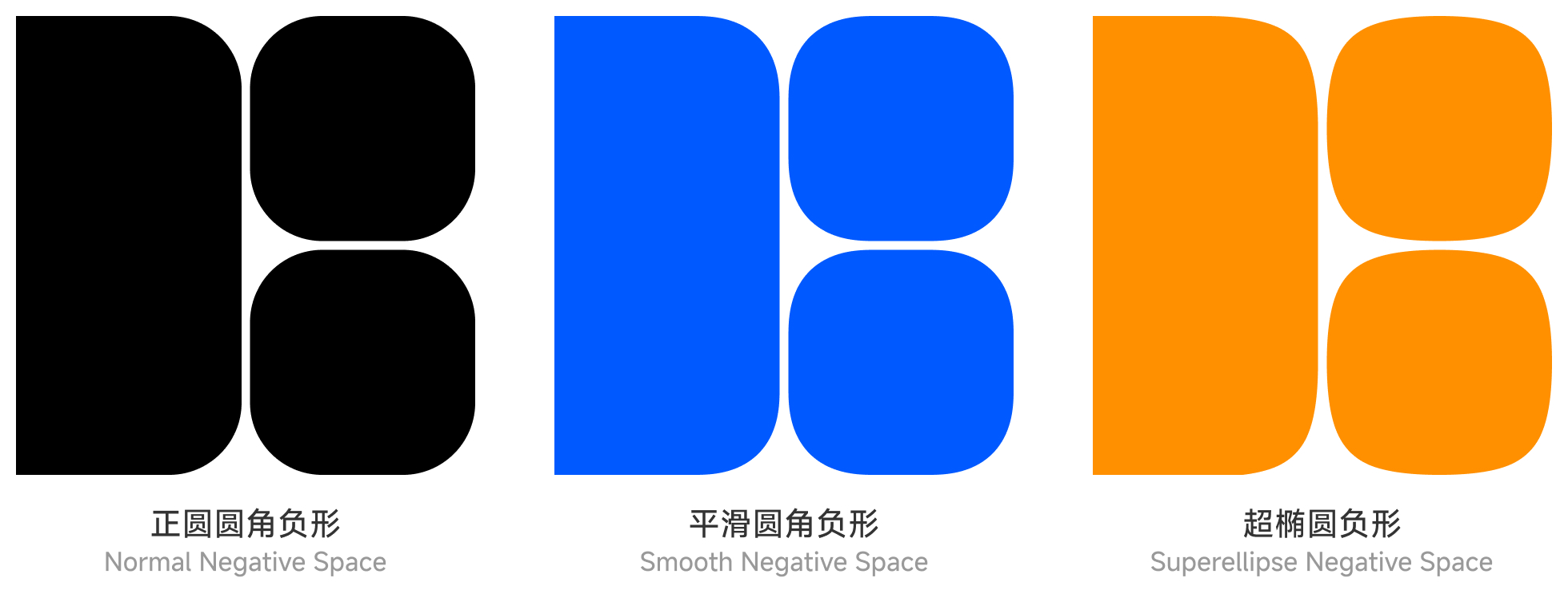
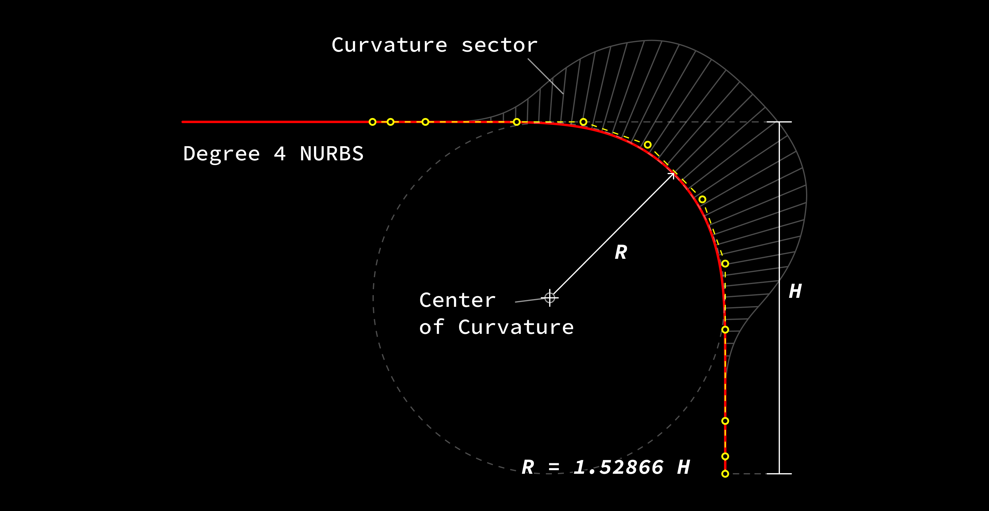
A superellipse is a natural candidate if mathematical smoothness is the only concern. But in system design, curves do not exist in isolation. The negative space formed by adjacent corners also affects how users perceive the platform's character. The final technical choice was therefore an engineering decision constrained by the design language.
Rasterization: Why SSAA?
Modern screens are pixel arrays, so vector curves ultimately have to be converted into pixels. There is no shortage of rasterization approaches. The real question is which approach is worth precomputing and caching once the corner shape has been fixed.
| Technique | Overview | Advantages | Disadvantages |
|---|---|---|---|
| SSAA (supersample anti-aliasing) | Render at a higher resolution, then downsample for smoother edges | Highest image quality, almost no jagged edges, broadly applicable | High processing and memory costs |
| MSAA (multisample anti-aliasing) | Take multiple samples at geometric boundaries to improve edge smoothness | Balances performance and quality; effective on geometric edges | Limited support for transparent textures and complex pixel effects |
| FXAA (fast approximate anti-aliasing) | Detect and blur edges in a pixel-shader post-processing pass | Very low cost, easy to integrate | Lost detail, blurred edges, limited results in high-contrast scenes |
| TAA (temporal anti-aliasing) | Sample and blend data from previous frames to reduce aliasing | Effective aliasing reduction; useful in dynamic scenes | Can introduce trails and ghosting, compromising results in motion |
| CMAA (conservative morphological anti-aliasing) | Combine edge detection and blending to balance performance and quality | Low cost, broad compatibility | Limited effectiveness; visible aliasing can remain in some scenes |
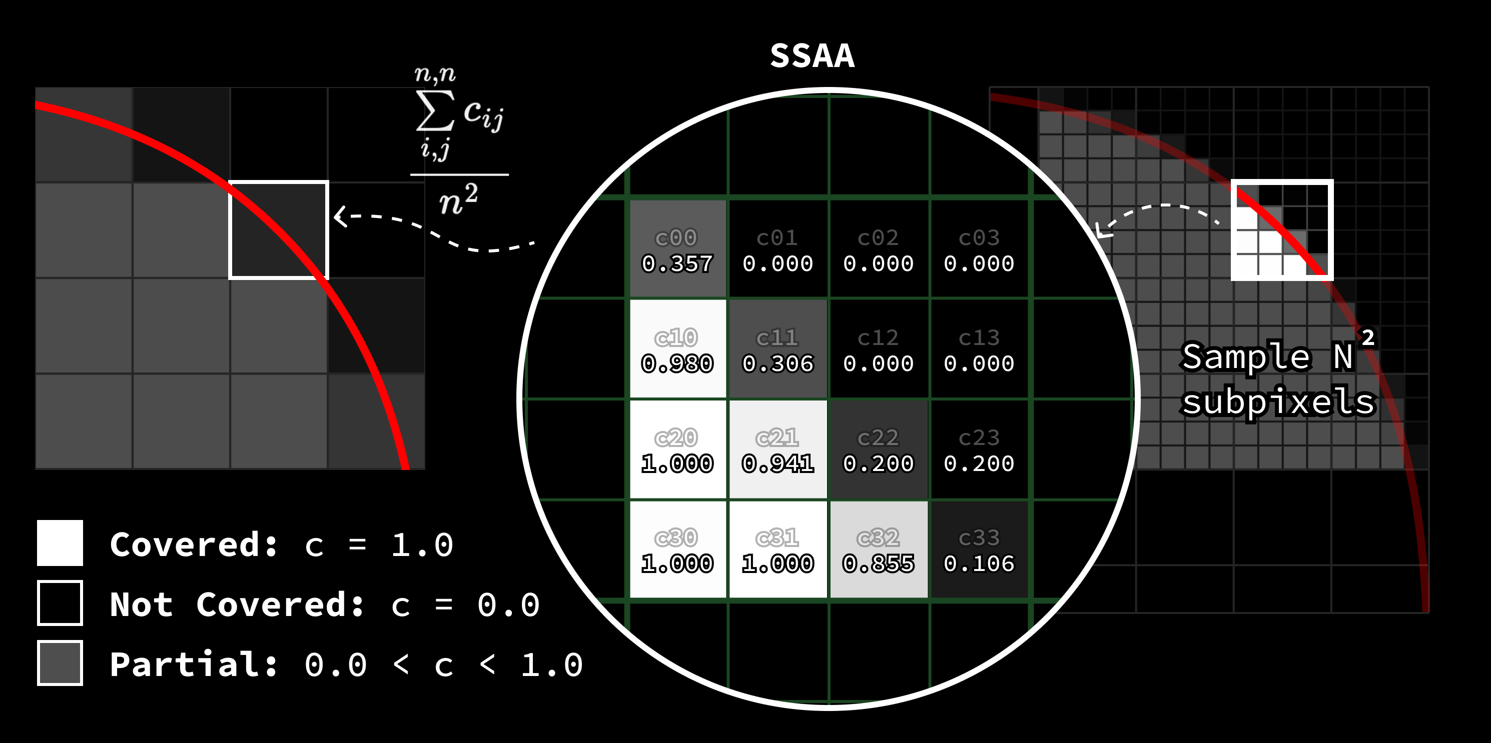
Because the corner shape is a cacheable system asset rather than complex geometry that changes every frame, we can choose SSAA for its image quality, rasterize once, and reuse the result. Moving this expensive, high-quality work into the caching stage substantially reduces its runtime burden.
Resampling: Why Lanczos and Nine Mipmap Levels?
A single high-resolution corner image does not solve every problem. Relying on a single cached image for large reductions at runtime produces visible aliasing because the sampling frequency no longer matches the image content.
This is why I approached it as a conventional texture-pipeline problem:
- Create a high-quality master image.
- Generate multiple mipmap levels.
- Sample at runtime from a level with a more suitable frequency range.
The following resampling algorithms were considered:
| Algorithm / Type | Method | Advantages | Disadvantages / Notes |
|---|---|---|---|
| Nearest neighbor | Take the pixel at the nearest integer coordinates, without interpolation | Hardware-supported; extremely fast and simple | Visible blocks and jagged edges; lowest quality |
| Bilinear | Linearly interpolate a weighted average of the surrounding 2x2 pixels | Hardware-supported; smooth and fast | Blurred edges and lost detail |
| Bicubic | Interpolate a 4x4 neighborhood using a cubic convolution kernel | Balances sharpness and smoothness, with good detail | More computation; possible mild ringing |
| Lanczos resampling (windowed sinc) | Interpolate a larger neighborhood, such as 6x6, using a windowed sinc kernel | Sharp results and excellent aliasing suppression | High cost; possible ringing |
| Mitchell–Netravali | Use an adjustable cubic kernel, commonly used for high-quality scaling | Balances detail and smoothness; suitable for content pipelines | Moderate algorithmic complexity |
| Area / Box | Average the input region covered by each output pixel, typically for downscaling | Fast, with good anti-aliasing when downscaling | Blurring and detail loss when upscaling |
| Gaussian | Blur with Gaussian weights, then sample | Natural smoothness and good aliasing suppression | Lost detail and relatively high computational cost |
| Catmull–Rom | Use a sharp cubic interpolation kernel, commonly used in content pipelines | Clear edges and good detail | Risk of ringing; moderate cost |
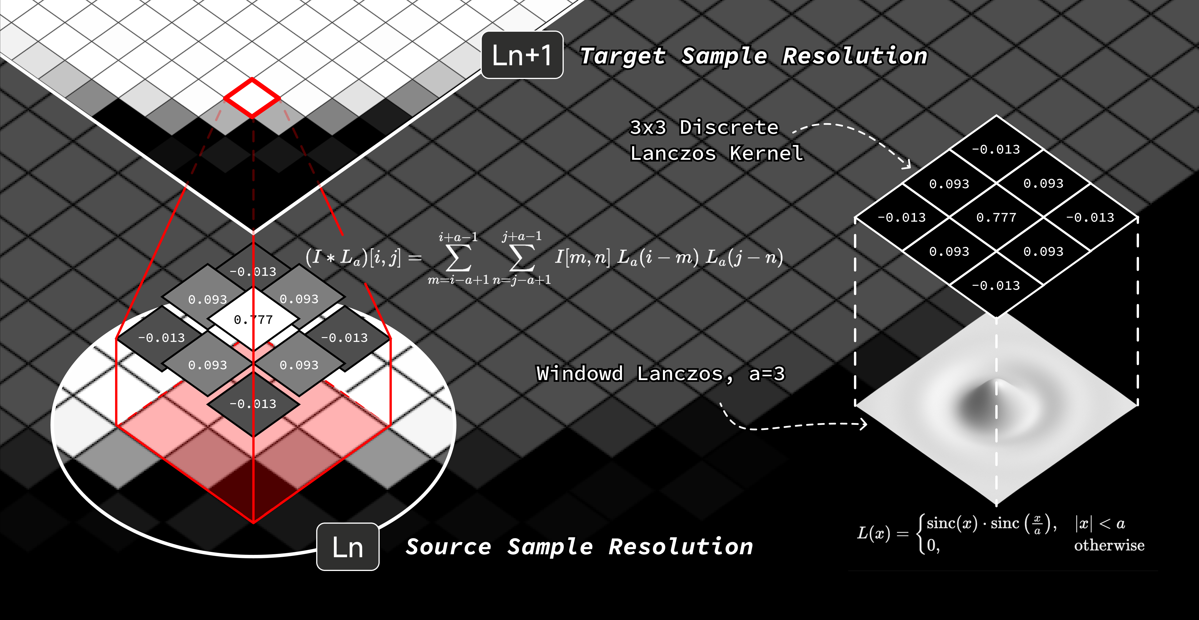
Lanczos was chosen for two reasons:
- It suppresses aliasing well enough to produce cleaner edges when downscaling.
- It preserves the original signal's shape more faithfully, rather than softening away the intended curvature relationships.
Using a window parameter of , we can convolve the original image with a normalized discrete Lanczos kernel to obtain the first resampled image :
Repeating the operation recursively on produces the remaining mipmap levels:
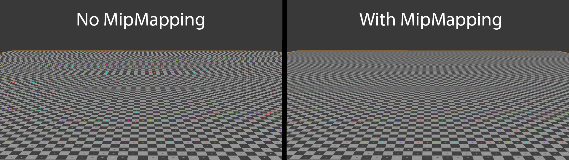
Multiple mipmap levels are necessary rather than directly reducing a single image. Otherwise, large scale reductions are more likely to produce moiré patterns.
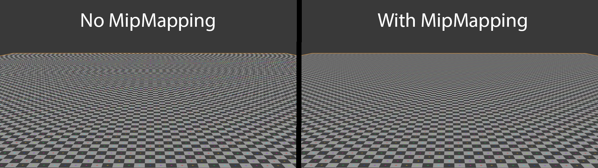
Image source: Wikimedia Commons.
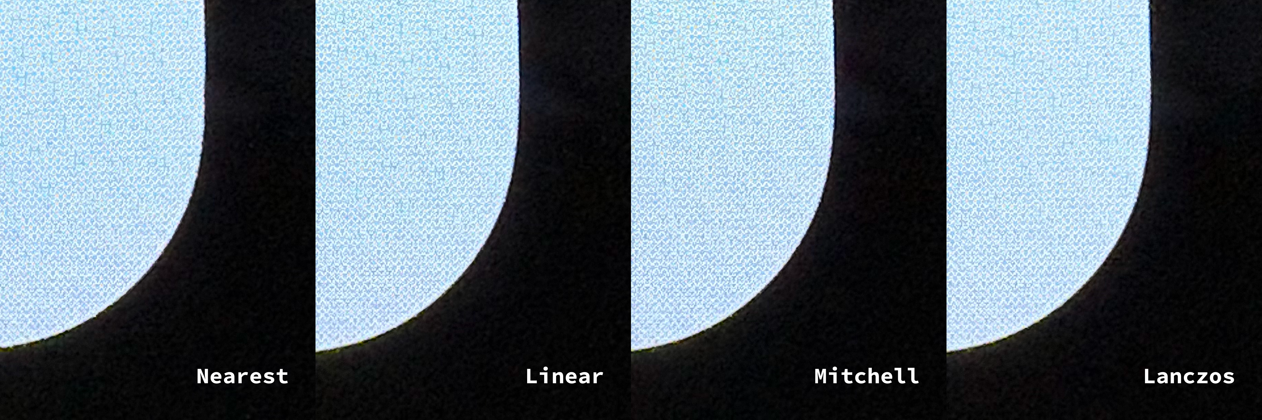
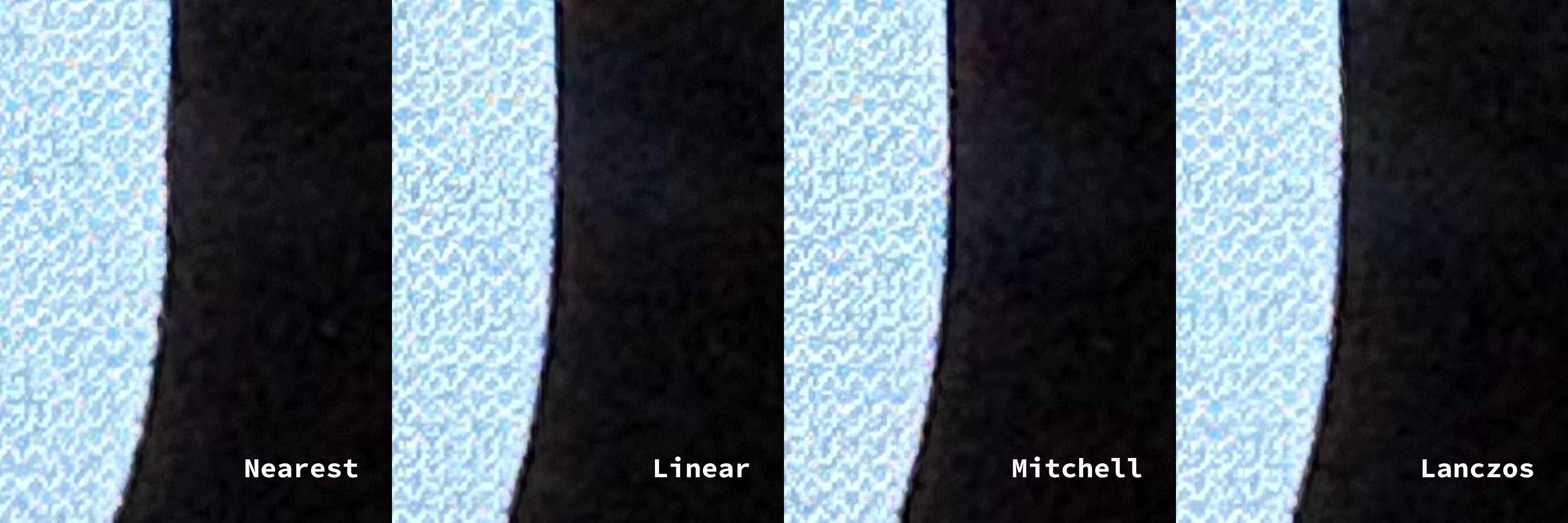
The on-device photographs below compare nearest-neighbor, linear, Mitchell, and Lanczos resampling. Nearest-neighbor and linear resampling show visible jaggedness. Mitchell and Lanczos are both sufficiently smooth, but further magnification shows that Lanczos better preserves the original curve's shape.
Runtime Sampling: Why Trilinear Filtering Is Enough
The final stage samples and filters the texture across the mipmap chain. Common options include:
| Filtering Method | Overview | Advantages | Disadvantages |
|---|---|---|---|
| Nearest neighbor | Use the color of the nearest pixel | Simple and fast | Visible aliasing and lost detail |
| Nearest neighbor with mipmapping | Combine nearest-neighbor sampling with multiple mipmap levels | Fast; reduces artifacts at a distance | Aliasing remains; abrupt transitions |
| Bilinear | Linearly interpolate the four pixels surrounding the sample point | Smooth edges and good performance | Blurred detail; artifacts can remain at a distance |
| Trilinear with mipmapping | Linearly interpolate between mipmap levels, using bilinear filtering within each level | Smooth transitions, with reduced aliasing and artifacts | Higher cost; detail remains limited |
| Anisotropic | Adapt sampling to the viewing angle to improve texture clarity at oblique angles and at a distance | Strong detail preservation; best results at oblique angles and at a distance | Higher cost and greater hardware requirements |
The primary target is mobile UI, not textures viewed at steep perspective angles, so anisotropic filtering offers little benefit for its cost. Trilinear filtering with mipmapping is a cost-effective final stage: image quality is already stable enough, and modern GPUs provide mature hardware support.
Results in Practice


Examining the display's subpixels under a microscope makes the improvement clear: the new corners transition more smoothly from straight edges into curves, largely eliminating the bump visible in the previous version.

Future Evolution
After more than three years of intermittent research and analysis of other industry implementations, high-performance smooth corners can now be described through a relatively stable technical architecture. If a better algorithm becomes available for an intermediate graphics stage, that stage can be replaced without rebuilding the entire pipeline.
For resampling, for example, convolution kernels such as John Costella's Magic Kernel may offer potential value on certain low-resolution devices. For me, the most important result is not the particular algorithm chosen for this release, but turning the rounded-corner problem into a graphics pipeline that can keep evolving.