Differentiable Polyphase Filter Optimization

September 01

Overview

This article uses a filtering chain based on Android Kawase V2 throughout. It starts by fitting a single-phase impulse response, examines the phase errors introduced by downsampling, and then introduces the polyphase supervision method from DPF: Differentiable Polyphase Filtering for Large-Kernel Approximation (SIGGRAPH 2026). Finally, it extends the optimization problem to downsampled blur with fixed, shared mipmap kernels, outlining how to solve for scale-dependent final sampling parameters under a fixed sampling budget.

Single-Phase Kawase Optimization

1. Shape Differences Between Kawase and Gaussian Blur

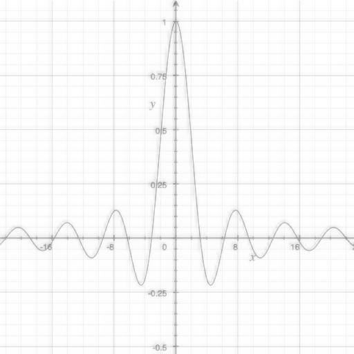
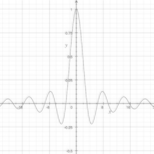
First, compare full-resolution Gaussian blur and Android Kawase V2 on the same 512×512512\times512 sinc test image, with their blur widths matched to target values of σ=4,8,16,40\sigma=4,8,16,40. The Dual Kawase implementation preserves high-frequency information by blending the original image with the blurred result. Its blur shape differs substantially from a Gaussian at the same scale.

Same 512×512 sinc test image · Outputs at 1× · RMSE in linear luminance
Methodσ = 4σ = 8σ = 16σ = 40
GaussianTarget σ=4, Gaussian actual sinc-image output

Image RMSE 0

Target σ=8, Gaussian actual sinc-image output

Image RMSE 0

Target σ=16, Gaussian actual sinc-image output

Image RMSE 0

Target σ=40, Gaussian actual sinc-image output

Image RMSE 0

Android Kawase V2Target σ=4, Android Kawase V2 blurRadius=6 actual sinc-image output

blurRadius=6
Matched σ≈3.9817
Image RMSE 5.722e-2

Target σ=8, Android Kawase V2 blurRadius=17 actual sinc-image output

blurRadius=17
Matched σ≈8.0894
Image RMSE 6.388e-3

Target σ=16, Android Kawase V2 blurRadius=32 actual sinc-image output

blurRadius=32
Matched σ≈16.0737
Image RMSE 4.239e-3

Target σ=40, Android Kawase V2 blurRadius=90 actual sinc-image output

blurRadius=90
Matched σ≈39.8502
Image RMSE 4.809e-3

2. The Kawase Processing Chain

The following diagram expands the Android Dual Kawase chain for a target of σ=4\sigma=4: an initial 4× downsample followed by one 2× downsample; on the way back, a 2× reconstruction blended with the saved image at that level, followed by a final 4× reconstruction blended with the original image.

Android Kawase V2 · σ=4 · blurRadius=6 · N=1 · SVG
Android Kawase V2 · σ=4 · blurRadius=6 · N=1 processing chainThe top row runs a 4× downsample and a 2× downsample from left to right, turning down at 64×64. The bottom row returns right to left with 2× reconstruction and same-level blending, then 4× reconstruction and original-image blending. Vertical dashed lines connect saved images to their blend stages.Original f → C_rSaved q₀ → M₀Input fFull resolution512 × 512Downsample 1 · ×4K_d,4q₀ · 128 × 128Downsample 2 · ×2K_d,2q₁ = p₁ · 64 × 64Upsample 1 · ×2K_u(s) → same-level blend M₀p₀ · 128 × 128Upsample 2 → blend C_r×4 · Triangle reconstruction b → blendOutput f′ · 512 × 512

Vertical dashed lines feed saved images from the top row into the blend stages below: Mᵢ(z) = αᵢ z + (1 − αᵢ) qᵢ; C_r(b) = β(r) b + (1 − β(r)) f.

The notation is as follows:

  • f(x)f(\mathbf x) and f′(x)f'(\mathbf x) are the full-resolution input and output. x\mathbf x denotes spatial coordinates before rearrangement, and k\mathbf k denotes discrete pixel indices after rearrangement. Intermediate stages use their respective input pixels as coordinate units.
  • UKu(s)\mathcal U_{K_u(s)} performs upsampling reconstruction with a sampling kernel. The Android implementation determines ss internally from blurRadius; p~i\widetilde p_i is the reconstructed image before blending.
  • Mi\mathcal M_i blends the reconstructed result with the previously saved downsampled image at the same level: Mi(z)=αiz+(1−αi)qi\mathcal M_i(z)=\alpha_i z+(1-\alpha_i)q_i.
  • Cr\mathcal C_r blends in the original image at small radii: Cr(z)=β(r)z+(1−β(r))f\mathcal C_r(z)=\beta(r)z+(1-\beta(r))f, where rr is the integer blurRadius and β(r)=min⁡(1,r/10)\beta(r)=\min(1,r/10).

For blurRadius=6, the intermediate images follow 5122→1282→642→1282→5122512^2\to128^2\to64^2\to128^2\to512^2.

Input
512 × 512
Android Kawase V2, blurRadius=6: Input
Fixed 4×4 downsampling
128 × 128
Android Kawase V2, blurRadius=6: Fixed 4×4 downsampling
2× downsampling 1
64 × 64
Android Kawase V2, blurRadius=6: 2× downsampling 1
2× upsampling 1 · Blend 0.3464
128 × 128
Android Kawase V2, blurRadius=6: 2× upsampling 1 · Blend 0.3464
4× enlargement + original blend
512 × 512
Android Kawase V2, blurRadius=6: 4× enlargement + original blend

At the return to 1282128^2, the inter-level blend factor is approximately 0.34640.3464. The final output contains 60%60\% blurred content and 40%40\% of the original image. Consequently, this small-radius result retains sharp details, and its impulse response contains a spike from the original-image contribution. It is not a strict Gaussian.

3. Single-Phase Impulse-Response Optimization

A common way to quantify the difference between Kawase and a reference blur kernel is to use the response to a single impulse as the equivalent convolution kernel of a complex graphics pipeline.

Input, Output, and Cross-Section

To evaluate a blur chain, construct a discrete impulse δ\delta: an image with a value of 11 at the center pixel and 00 everywhere else. Pass it through the complete processing chain P\mathcal P and record the output weight distribution:

K=P(δ).K=\mathcal P(\delta).

The resulting KK is the impulse response at that input location. Its 2D image and center-row cross-section reveal its spread, peak, and shape. Comparing it with the target Gaussian also gives error metrics for parameter tuning. Below, Android Kawase V2 (blurRadius=90) processes a unit impulse at phase (0,0)(0,0). The full-resolution Gaussian is the reference, with the target scale still set to σ=40\sigma=40.

Input
Discrete unit impulse at the center pixel, with the central region enlarged using nearest-neighbor sampling

Discrete impulse δ\delta (enlarged center)

Gaussian
Gaussian full phase-zero impulse response, shared display gain 2500×AA05.4e-51.1e-4-2400240

A—A · Position relative to input / px

Android Kawase V2
Android Kawase V2 full phase-zero impulse response, shared display gain 2500×AA05.4e-51.1e-4-2400240

A—A · Position relative to input / px

A—A marks the cross-section. The overlaid curve below shows its raw values; the gray dashed curve is the Gaussian reference.

This approach to kernel evaluation is called single-impulse evaluation.

Although the Kawase baseline has a support size similar to the reference Gaussian, its peak is noticeably lower and its shape is flatter. Visually, the result looks somewhat “square.”

Single-Impulse Evaluation and the LSI Condition

The theoretical basis for single-impulse evaluation is the behavior of linear shift-invariant systems (LSI). If P\mathcal P is both linear and shift-invariant, one impulse response determines its output for any input:

P(δ)=K⟹∀f,  P(f)=f∗K.\mathcal P(\delta)=K \quad\Longrightarrow\quad \forall f,\;\mathcal P(f)=f\ast K.

In that case, optimizing the impulse response is equivalent to optimizing the convolution kernel of the entire chain. Dual Kawase, however, is not an LSI system. This is the central issue explored in this article. For now, we follow the single-impulse approach and fit the Dual Kawase response at one location to a Gaussian as closely as possible. The next section introduces a method that addresses the missing supervision.

Defining the Optimization Variables

The kernels at each stage are shown below. Offsets are measured in input texels of the corresponding pass, and every lookup uses bilinear sampling.

Kd,4 · 4× downsampling
Four diagonal taps · 1/4 per sample
Input pixel center (-2.5, -2.5), accumulated weight at the reference alignment: 0.000000Input pixel center (-1.5, -2.5), accumulated weight at the reference alignment: 0.000000Input pixel center (-0.5, -2.5), accumulated weight at the reference alignment: 0.000000Input pixel center (0.5, -2.5), accumulated weight at the reference alignment: 0.000000Input pixel center (1.5, -2.5), accumulated weight at the reference alignment: 0.000000Input pixel center (2.5, -2.5), accumulated weight at the reference alignment: 0.000000Input pixel center (-2.5, -1.5), accumulated weight at the reference alignment: 0.000000Input pixel center (-1.5, -1.5), accumulated weight at the reference alignment: 0.062500Input pixel center (-0.5, -1.5), accumulated weight at the reference alignment: 0.062500Input pixel center (0.5, -1.5), accumulated weight at the reference alignment: 0.062500Input pixel center (1.5, -1.5), accumulated weight at the reference alignment: 0.062500Input pixel center (2.5, -1.5), accumulated weight at the reference alignment: 0.000000Input pixel center (-2.5, -0.5), accumulated weight at the reference alignment: 0.000000Input pixel center (-1.5, -0.5), accumulated weight at the reference alignment: 0.062500Input pixel center (-0.5, -0.5), accumulated weight at the reference alignment: 0.062500Input pixel center (0.5, -0.5), accumulated weight at the reference alignment: 0.062500Input pixel center (1.5, -0.5), accumulated weight at the reference alignment: 0.062500Input pixel center (2.5, -0.5), accumulated weight at the reference alignment: 0.000000Input pixel center (-2.5, 0.5), accumulated weight at the reference alignment: 0.000000Input pixel center (-1.5, 0.5), accumulated weight at the reference alignment: 0.062500Input pixel center (-0.5, 0.5), accumulated weight at the reference alignment: 0.062500Input pixel center (0.5, 0.5), accumulated weight at the reference alignment: 0.062500Input pixel center (1.5, 0.5), accumulated weight at the reference alignment: 0.062500Input pixel center (2.5, 0.5), accumulated weight at the reference alignment: 0.000000Input pixel center (-2.5, 1.5), accumulated weight at the reference alignment: 0.000000Input pixel center (-1.5, 1.5), accumulated weight at the reference alignment: 0.062500Input pixel center (-0.5, 1.5), accumulated weight at the reference alignment: 0.062500Input pixel center (0.5, 1.5), accumulated weight at the reference alignment: 0.062500Input pixel center (1.5, 1.5), accumulated weight at the reference alignment: 0.062500Input pixel center (2.5, 1.5), accumulated weight at the reference alignment: 0.000000Input pixel center (-2.5, 2.5), accumulated weight at the reference alignment: 0.000000Input pixel center (-1.5, 2.5), accumulated weight at the reference alignment: 0.000000Input pixel center (-0.5, 2.5), accumulated weight at the reference alignment: 0.000000Input pixel center (0.5, 2.5), accumulated weight at the reference alignment: 0.000000Input pixel center (1.5, 2.5), accumulated weight at the reference alignment: 0.000000Input pixel center (2.5, 2.5), accumulated weight at the reference alignment: 0.000000-2-2-1-1001122ΔxΔyOffset from sampling center (1, 1) input texels, weight 1/4Offset from sampling center (1, -1) input texels, weight 1/4Offset from sampling center (-1, -1) input texels, weight 1/4Offset from sampling center (-1, 1) input texels, weight 1/4

Offset / input texels

Kd,2 · 2× downsampling
Center 1/2 · Four diagonal taps at 1/8 each
Input pixel center (-2.5, -2.5), accumulated weight at the reference alignment: 0.000000Input pixel center (-1.5, -2.5), accumulated weight at the reference alignment: 0.000000Input pixel center (-0.5, -2.5), accumulated weight at the reference alignment: 0.000000Input pixel center (0.5, -2.5), accumulated weight at the reference alignment: 0.000000Input pixel center (1.5, -2.5), accumulated weight at the reference alignment: 0.000000Input pixel center (2.5, -2.5), accumulated weight at the reference alignment: 0.000000Input pixel center (-2.5, -1.5), accumulated weight at the reference alignment: 0.000000Input pixel center (-1.5, -1.5), accumulated weight at the reference alignment: 0.031250Input pixel center (-0.5, -1.5), accumulated weight at the reference alignment: 0.031250Input pixel center (0.5, -1.5), accumulated weight at the reference alignment: 0.031250Input pixel center (1.5, -1.5), accumulated weight at the reference alignment: 0.031250Input pixel center (2.5, -1.5), accumulated weight at the reference alignment: 0.000000Input pixel center (-2.5, -0.5), accumulated weight at the reference alignment: 0.000000Input pixel center (-1.5, -0.5), accumulated weight at the reference alignment: 0.031250Input pixel center (-0.5, -0.5), accumulated weight at the reference alignment: 0.156250Input pixel center (0.5, -0.5), accumulated weight at the reference alignment: 0.156250Input pixel center (1.5, -0.5), accumulated weight at the reference alignment: 0.031250Input pixel center (2.5, -0.5), accumulated weight at the reference alignment: 0.000000Input pixel center (-2.5, 0.5), accumulated weight at the reference alignment: 0.000000Input pixel center (-1.5, 0.5), accumulated weight at the reference alignment: 0.031250Input pixel center (-0.5, 0.5), accumulated weight at the reference alignment: 0.156250Input pixel center (0.5, 0.5), accumulated weight at the reference alignment: 0.156250Input pixel center (1.5, 0.5), accumulated weight at the reference alignment: 0.031250Input pixel center (2.5, 0.5), accumulated weight at the reference alignment: 0.000000Input pixel center (-2.5, 1.5), accumulated weight at the reference alignment: 0.000000Input pixel center (-1.5, 1.5), accumulated weight at the reference alignment: 0.031250Input pixel center (-0.5, 1.5), accumulated weight at the reference alignment: 0.031250Input pixel center (0.5, 1.5), accumulated weight at the reference alignment: 0.031250Input pixel center (1.5, 1.5), accumulated weight at the reference alignment: 0.031250Input pixel center (2.5, 1.5), accumulated weight at the reference alignment: 0.000000Input pixel center (-2.5, 2.5), accumulated weight at the reference alignment: 0.000000Input pixel center (-1.5, 2.5), accumulated weight at the reference alignment: 0.000000Input pixel center (-0.5, 2.5), accumulated weight at the reference alignment: 0.000000Input pixel center (0.5, 2.5), accumulated weight at the reference alignment: 0.000000Input pixel center (1.5, 2.5), accumulated weight at the reference alignment: 0.000000Input pixel center (2.5, 2.5), accumulated weight at the reference alignment: 0.000000-2-2-1-1001122ΔxΔyOffset from sampling center (0, 0) input texels, weight 1/2Offset from sampling center (1, 1) input texels, weight 1/8Offset from sampling center (1, -1) input texels, weight 1/8Offset from sampling center (-1, -1) input texels, weight 1/8Offset from sampling center (-1, 1) input texels, weight 1/8

Offset / input texels

Ku(s) · 2× upsampling
Center + regular heptagon · 1/8 per sample
Input pixel center (-2.5, -2.5), accumulated weight at the reference alignment: 0.000000Input pixel center (-1.5, -2.5), accumulated weight at the reference alignment: 0.000000Input pixel center (-0.5, -2.5), accumulated weight at the reference alignment: 0.000000Input pixel center (0.5, -2.5), accumulated weight at the reference alignment: 0.000000Input pixel center (1.5, -2.5), accumulated weight at the reference alignment: 0.000000Input pixel center (2.5, -2.5), accumulated weight at the reference alignment: 0.000000Input pixel center (-2.5, -1.5), accumulated weight at the reference alignment: 0.000000Input pixel center (-1.5, -1.5), accumulated weight at the reference alignment: 0.000000Input pixel center (-0.5, -1.5), accumulated weight at the reference alignment: 0.042893Input pixel center (0.5, -1.5), accumulated weight at the reference alignment: 0.047351Input pixel center (1.5, -1.5), accumulated weight at the reference alignment: 0.004350Input pixel center (2.5, -1.5), accumulated weight at the reference alignment: 0.000000Input pixel center (-2.5, -0.5), accumulated weight at the reference alignment: 0.000000Input pixel center (-1.5, -0.5), accumulated weight at the reference alignment: 0.050121Input pixel center (-0.5, -0.5), accumulated weight at the reference alignment: 0.153551Input pixel center (0.5, -0.5), accumulated weight at the reference alignment: 0.159397Input pixel center (1.5, -0.5), accumulated weight at the reference alignment: 0.042336Input pixel center (2.5, -0.5), accumulated weight at the reference alignment: 0.000000Input pixel center (-2.5, 0.5), accumulated weight at the reference alignment: 0.000000Input pixel center (-1.5, 0.5), accumulated weight at the reference alignment: 0.050121Input pixel center (-0.5, 0.5), accumulated weight at the reference alignment: 0.153551Input pixel center (0.5, 0.5), accumulated weight at the reference alignment: 0.159397Input pixel center (1.5, 0.5), accumulated weight at the reference alignment: 0.042336Input pixel center (2.5, 0.5), accumulated weight at the reference alignment: 0.000000Input pixel center (-2.5, 1.5), accumulated weight at the reference alignment: 0.000000Input pixel center (-1.5, 1.5), accumulated weight at the reference alignment: 0.000000Input pixel center (-0.5, 1.5), accumulated weight at the reference alignment: 0.042893Input pixel center (0.5, 1.5), accumulated weight at the reference alignment: 0.047351Input pixel center (1.5, 1.5), accumulated weight at the reference alignment: 0.004350Input pixel center (2.5, 1.5), accumulated weight at the reference alignment: 0.000000Input pixel center (-2.5, 2.5), accumulated weight at the reference alignment: 0.000000Input pixel center (-1.5, 2.5), accumulated weight at the reference alignment: 0.000000Input pixel center (-0.5, 2.5), accumulated weight at the reference alignment: 0.000000Input pixel center (0.5, 2.5), accumulated weight at the reference alignment: 0.000000Input pixel center (1.5, 2.5), accumulated weight at the reference alignment: 0.000000Input pixel center (2.5, 2.5), accumulated weight at the reference alignment: 0.000000-2-2-1-1001122ΔxΔyOffset from sampling center (0, 0) input texels, weight 1/8Offset from sampling center (1, 0) input texels, weight 1/8Offset from sampling center (0.623489802, 0.781831482) input texels, weight 1/8Offset from sampling center (-0.222520934, 0.974927912) input texels, weight 1/8Offset from sampling center (-0.900968868, 0.433883739) input texels, weight 1/8Offset from sampling center (-0.900968868, -0.433883739) input texels, weight 1/8Offset from sampling center (-0.222520934, -0.974927912) input texels, weight 1/8Offset from sampling center (0.623489802, -0.781831482) input texels, weight 1/8

Offset / input texels

All three kernel diagrams place the sampling center at the intersection of four input pixels. Squares represent complete input pixels, dots mark pixel centers, and hollow circles mark the stencil's sample positions. Coordinates are relative to the sampling center, with Δx pointing right and Δy pointing down, matching the implementation. Gray intensity represents accumulated pixel weights at this reference alignment, with a shared scale across all three diagrams. One complete ring of pixels is retained around the coverage area. The upsampling example uses s=2 (a=s/2=1); the dashed circle has radius a. These are reference diagrams of the kernel stencils, not actual output phases. During execution, the sampling center's alignment with the input pixels varies with the output phase, as do the interpolation weights.

These three kernels can be described by four variables: starting angle θ\theta, number of outer samples nn, center weight wcw_c, and ring radius aa.

Adjustable Sampling Kernel
Input pixel center (-2.5, -2.5), accumulated weight at the reference alignment: 0.000000Input pixel center (-1.5, -2.5), accumulated weight at the reference alignment: 0.000000Input pixel center (-0.5, -2.5), accumulated weight at the reference alignment: 0.000000Input pixel center (0.5, -2.5), accumulated weight at the reference alignment: 0.000000Input pixel center (1.5, -2.5), accumulated weight at the reference alignment: 0.000000Input pixel center (2.5, -2.5), accumulated weight at the reference alignment: 0.000000Input pixel center (-2.5, -1.5), accumulated weight at the reference alignment: 0.000000Input pixel center (-1.5, -1.5), accumulated weight at the reference alignment: 0.031250Input pixel center (-0.5, -1.5), accumulated weight at the reference alignment: 0.031250Input pixel center (0.5, -1.5), accumulated weight at the reference alignment: 0.031250Input pixel center (1.5, -1.5), accumulated weight at the reference alignment: 0.031250Input pixel center (2.5, -1.5), accumulated weight at the reference alignment: 0.000000Input pixel center (-2.5, -0.5), accumulated weight at the reference alignment: 0.000000Input pixel center (-1.5, -0.5), accumulated weight at the reference alignment: 0.031250Input pixel center (-0.5, -0.5), accumulated weight at the reference alignment: 0.156250Input pixel center (0.5, -0.5), accumulated weight at the reference alignment: 0.156250Input pixel center (1.5, -0.5), accumulated weight at the reference alignment: 0.031250Input pixel center (2.5, -0.5), accumulated weight at the reference alignment: 0.000000Input pixel center (-2.5, 0.5), accumulated weight at the reference alignment: 0.000000Input pixel center (-1.5, 0.5), accumulated weight at the reference alignment: 0.031250Input pixel center (-0.5, 0.5), accumulated weight at the reference alignment: 0.156250Input pixel center (0.5, 0.5), accumulated weight at the reference alignment: 0.156250Input pixel center (1.5, 0.5), accumulated weight at the reference alignment: 0.031250Input pixel center (2.5, 0.5), accumulated weight at the reference alignment: 0.000000Input pixel center (-2.5, 1.5), accumulated weight at the reference alignment: 0.000000Input pixel center (-1.5, 1.5), accumulated weight at the reference alignment: 0.031250Input pixel center (-0.5, 1.5), accumulated weight at the reference alignment: 0.031250Input pixel center (0.5, 1.5), accumulated weight at the reference alignment: 0.031250Input pixel center (1.5, 1.5), accumulated weight at the reference alignment: 0.031250Input pixel center (2.5, 1.5), accumulated weight at the reference alignment: 0.000000Input pixel center (-2.5, 2.5), accumulated weight at the reference alignment: 0.000000Input pixel center (-1.5, 2.5), accumulated weight at the reference alignment: 0.000000Input pixel center (-0.5, 2.5), accumulated weight at the reference alignment: 0.000000Input pixel center (0.5, 2.5), accumulated weight at the reference alignment: 0.000000Input pixel center (1.5, 2.5), accumulated weight at the reference alignment: 0.000000Input pixel center (2.5, 2.5), accumulated weight at the reference alignment: 0.000000-4-4-3-3-2-2-1-10011223344ΔxΔyOffset from sampling center (0, 0) input texels, weight 0.5Offset from sampling center (1.0000000000000002, 1) input texels, weight 0.125Offset from sampling center (-1, 1.0000000000000002) input texels, weight 0.125Offset from sampling center (-1.0000000000000002, -1) input texels, weight 0.125Offset from sampling center (0.9999999999999998, -1.0000000000000002) input texels, weight 0.125
°
texel
Weight per outer tap 0.1250

Offset / input texels

The nn outer points are evenly spaced on a circle of radius aa. Point ii has angle θ+2πi/n\theta+2\pi i/n and weight (1−wc)/n(1-w_c)/n; the center has weight wcw_c. Drag the sliders or enter values to inspect the sample positions and bilinear interpolation weights. The sampling center remains at the intersection of four input pixels, the grayscale scale is fixed, and the coordinate range includes every affected pixel. Faint hollow dots indicate zero-weight samples.

For the three Kawase downsampling and upsampling kernels above:

KernelStarting angle θ\thetaOuter samples nnCenter weight wcw_cRing radius aa
Kd,4K_{d,4}π/4\pi/444002\sqrt{2}
Kd,2K_{d,2}π/4\pi/4441/21/22\sqrt{2}
Ku(s)K_u(s)00771/81/8s/2s/2

There are also the inter-level blend factor α\alpha and the final blurred-image fraction β\beta. For the σ=4\sigma=4 chain below, the three kernels have four parameters each. With the two blend factors, this gives 3×4+2=143\times4+2=14 parameters. The three sample counts nn are discrete integers, fixed here to 4,4,74,4,7. The continuous optimization therefore uses (θ,wc,a)(\theta,w_c,a) for each kernel, plus α,β\alpha,\beta: 3×3+2=113\times3+2=11 variables. For convenience, write each kernel's parameter group as Ωk=(θk,nk,wc,k,ak)\Omega_k=(\theta_k,n_k,w_{c,k},a_k), with kk taking the values d,4d,4, d,2d,2, and uu. A complete solution is Ω=(Ωd,4,Ωd,2,Ωu,α,β)\Omega=(\Omega_{d,4},\Omega_{d,2},\Omega_u,\alpha,\beta).

Defining the Single-Phase Loss and Solving with Gradients

Let GσG_\sigma be the full-resolution discrete Gaussian kernel with target standard deviation σ\sigma, and let FΩ\mathcal F_\Omega denote the complete Kawase chain. Place a unit impulse δ0\delta_0 at the fixed center location, phase (0,0)(0,0), and minimize the squared error against the target response:

Lsingle(Ω)=∥FΩ(δ0)−Gσ∥22.\mathcal L_{\mathrm{single}}(\Omega) =\left\|\mathcal F_{\Omega}(\delta_0)-G_\sigma\right\|_2^2.Ω∗≈arg min⁡Ω  Lsingle(Ω).\Omega^\ast \approx\underset{\Omega}{\operatorname{arg\,min}}\; \mathcal L_{\mathrm{single}}(\Omega).

Let DKd,4,4\mathcal D_{K_{d,4},4} and DKd,2,2\mathcal D_{K_{d,2},2} denote 4× and 2× downsampling with their respective kernels, UKu,2\mathcal U_{K_u,2} denote 2× upsampling with its kernel, and R4\mathcal R_4 denote fixed 4× bilinear reconstruction. For input ff, the intermediate images and two blends are

q0=DKd,4,4(f),q1=DKd,2,2(q0),p~0=UKu,2(q1),p0=(1−α)q0+αp~0,f′=(1−β)f+β R4(p0).\begin{aligned} q_0&=\mathcal D_{K_{d,4},4}(f), & q_1&=\mathcal D_{K_{d,2},2}(q_0),\\ \widetilde p_0&=\mathcal U_{K_u,2}(q_1), & p_0&=(1-\alpha)q_0+\alpha\widetilde p_0,\\ f'&=(1-\beta)f+\beta\,\mathcal R_4(p_0). \end{aligned}

p~0\widetilde p_0 is the reconstructed, pre-blend image described in the processing-chain section. When f=δ0f=\delta_0, the output f′f' is the FΩ(δ0)\mathcal F_\Omega(\delta_0) used in the loss.

The interactive demo below defaults to Levenberg–Marquardt (LM). It uses each output pixel's derivatives with respect to the parameters to estimate parameter sensitivities and interactions, then solves for a joint update direction. For background, see Ceres's explanation of LM.

λ 1.00e+0 · 0 rejected stepsStep 0 / 200 · Loss 35.059086
Kd,4 · 4× downsampling
n=4 · Used once · Three optimized parameters
Input pixel center (-2.5, -2.5), accumulated weight at the reference alignment: 0.000000Input pixel center (-1.5, -2.5), accumulated weight at the reference alignment: 0.000000Input pixel center (-0.5, -2.5), accumulated weight at the reference alignment: 0.000000Input pixel center (0.5, -2.5), accumulated weight at the reference alignment: 0.000000Input pixel center (1.5, -2.5), accumulated weight at the reference alignment: 0.000000Input pixel center (2.5, -2.5), accumulated weight at the reference alignment: 0.000000Input pixel center (-2.5, -1.5), accumulated weight at the reference alignment: 0.000000Input pixel center (-1.5, -1.5), accumulated weight at the reference alignment: 0.062500Input pixel center (-0.5, -1.5), accumulated weight at the reference alignment: 0.062500Input pixel center (0.5, -1.5), accumulated weight at the reference alignment: 0.062500Input pixel center (1.5, -1.5), accumulated weight at the reference alignment: 0.062500Input pixel center (2.5, -1.5), accumulated weight at the reference alignment: 0.000000Input pixel center (-2.5, -0.5), accumulated weight at the reference alignment: 0.000000Input pixel center (-1.5, -0.5), accumulated weight at the reference alignment: 0.062500Input pixel center (-0.5, -0.5), accumulated weight at the reference alignment: 0.062500Input pixel center (0.5, -0.5), accumulated weight at the reference alignment: 0.062500Input pixel center (1.5, -0.5), accumulated weight at the reference alignment: 0.062500Input pixel center (2.5, -0.5), accumulated weight at the reference alignment: 0.000000Input pixel center (-2.5, 0.5), accumulated weight at the reference alignment: 0.000000Input pixel center (-1.5, 0.5), accumulated weight at the reference alignment: 0.062500Input pixel center (-0.5, 0.5), accumulated weight at the reference alignment: 0.062500Input pixel center (0.5, 0.5), accumulated weight at the reference alignment: 0.062500Input pixel center (1.5, 0.5), accumulated weight at the reference alignment: 0.062500Input pixel center (2.5, 0.5), accumulated weight at the reference alignment: 0.000000Input pixel center (-2.5, 1.5), accumulated weight at the reference alignment: 0.000000Input pixel center (-1.5, 1.5), accumulated weight at the reference alignment: 0.062500Input pixel center (-0.5, 1.5), accumulated weight at the reference alignment: 0.062500Input pixel center (0.5, 1.5), accumulated weight at the reference alignment: 0.062500Input pixel center (1.5, 1.5), accumulated weight at the reference alignment: 0.062500Input pixel center (2.5, 1.5), accumulated weight at the reference alignment: 0.000000Input pixel center (-2.5, 2.5), accumulated weight at the reference alignment: 0.000000Input pixel center (-1.5, 2.5), accumulated weight at the reference alignment: 0.000000Input pixel center (-0.5, 2.5), accumulated weight at the reference alignment: 0.000000Input pixel center (0.5, 2.5), accumulated weight at the reference alignment: 0.000000Input pixel center (1.5, 2.5), accumulated weight at the reference alignment: 0.000000Input pixel center (2.5, 2.5), accumulated weight at the reference alignment: 0.000000-4-4-3-3-2-2-1-10011223344ΔxΔyOffset from sampling center (0, 0) input texels, weight 0Offset from sampling center (1.0000000000000002, 1) input texels, weight 0.25Offset from sampling center (-1, 1.0000000000000002) input texels, weight 0.25Offset from sampling center (-1.0000000000000002, -1) input texels, weight 0.25Offset from sampling center (0.9999999999999998, -1.0000000000000002) input texels, weight 0.25
Offset / input texels
Kd,2 · 2× downsampling
n=4 · Used once · Three optimized parameters
Input pixel center (-2.5, -2.5), accumulated weight at the reference alignment: 0.000000Input pixel center (-1.5, -2.5), accumulated weight at the reference alignment: 0.000000Input pixel center (-0.5, -2.5), accumulated weight at the reference alignment: 0.000000Input pixel center (0.5, -2.5), accumulated weight at the reference alignment: 0.000000Input pixel center (1.5, -2.5), accumulated weight at the reference alignment: 0.000000Input pixel center (2.5, -2.5), accumulated weight at the reference alignment: 0.000000Input pixel center (-2.5, -1.5), accumulated weight at the reference alignment: 0.000000Input pixel center (-1.5, -1.5), accumulated weight at the reference alignment: 0.031250Input pixel center (-0.5, -1.5), accumulated weight at the reference alignment: 0.031250Input pixel center (0.5, -1.5), accumulated weight at the reference alignment: 0.031250Input pixel center (1.5, -1.5), accumulated weight at the reference alignment: 0.031250Input pixel center (2.5, -1.5), accumulated weight at the reference alignment: 0.000000Input pixel center (-2.5, -0.5), accumulated weight at the reference alignment: 0.000000Input pixel center (-1.5, -0.5), accumulated weight at the reference alignment: 0.031250Input pixel center (-0.5, -0.5), accumulated weight at the reference alignment: 0.156250Input pixel center (0.5, -0.5), accumulated weight at the reference alignment: 0.156250Input pixel center (1.5, -0.5), accumulated weight at the reference alignment: 0.031250Input pixel center (2.5, -0.5), accumulated weight at the reference alignment: 0.000000Input pixel center (-2.5, 0.5), accumulated weight at the reference alignment: 0.000000Input pixel center (-1.5, 0.5), accumulated weight at the reference alignment: 0.031250Input pixel center (-0.5, 0.5), accumulated weight at the reference alignment: 0.156250Input pixel center (0.5, 0.5), accumulated weight at the reference alignment: 0.156250Input pixel center (1.5, 0.5), accumulated weight at the reference alignment: 0.031250Input pixel center (2.5, 0.5), accumulated weight at the reference alignment: 0.000000Input pixel center (-2.5, 1.5), accumulated weight at the reference alignment: 0.000000Input pixel center (-1.5, 1.5), accumulated weight at the reference alignment: 0.031250Input pixel center (-0.5, 1.5), accumulated weight at the reference alignment: 0.031250Input pixel center (0.5, 1.5), accumulated weight at the reference alignment: 0.031250Input pixel center (1.5, 1.5), accumulated weight at the reference alignment: 0.031250Input pixel center (2.5, 1.5), accumulated weight at the reference alignment: 0.000000Input pixel center (-2.5, 2.5), accumulated weight at the reference alignment: 0.000000Input pixel center (-1.5, 2.5), accumulated weight at the reference alignment: 0.000000Input pixel center (-0.5, 2.5), accumulated weight at the reference alignment: 0.000000Input pixel center (0.5, 2.5), accumulated weight at the reference alignment: 0.000000Input pixel center (1.5, 2.5), accumulated weight at the reference alignment: 0.000000Input pixel center (2.5, 2.5), accumulated weight at the reference alignment: 0.000000-4-4-3-3-2-2-1-10011223344ΔxΔyOffset from sampling center (0, 0) input texels, weight 0.5Offset from sampling center (1.0000000000000002, 1) input texels, weight 0.125Offset from sampling center (-1, 1.0000000000000002) input texels, weight 0.125Offset from sampling center (-1.0000000000000002, -1) input texels, weight 0.125Offset from sampling center (0.9999999999999998, -1.0000000000000002) input texels, weight 0.125
Offset / input texels
Ku(s) · 2× upsampling
n=7 · Used once · Three optimized parameters
Input pixel center (-2.5, -2.5), accumulated weight at the reference alignment: 0.000000Input pixel center (-1.5, -2.5), accumulated weight at the reference alignment: 0.000000Input pixel center (-0.5, -2.5), accumulated weight at the reference alignment: 0.000000Input pixel center (0.5, -2.5), accumulated weight at the reference alignment: 0.000000Input pixel center (1.5, -2.5), accumulated weight at the reference alignment: 0.000000Input pixel center (2.5, -2.5), accumulated weight at the reference alignment: 0.000000Input pixel center (-2.5, -1.5), accumulated weight at the reference alignment: 0.000000Input pixel center (-1.5, -1.5), accumulated weight at the reference alignment: 0.001466Input pixel center (-0.5, -1.5), accumulated weight at the reference alignment: 0.065174Input pixel center (0.5, -1.5), accumulated weight at the reference alignment: 0.060638Input pixel center (1.5, -1.5), accumulated weight at the reference alignment: 0.013534Input pixel center (2.5, -1.5), accumulated weight at the reference alignment: 0.000000Input pixel center (-2.5, -0.5), accumulated weight at the reference alignment: 0.000000Input pixel center (-1.5, -0.5), accumulated weight at the reference alignment: 0.071062Input pixel center (-0.5, -0.5), accumulated weight at the reference alignment: 0.114398Input pixel center (0.5, -0.5), accumulated weight at the reference alignment: 0.112636Input pixel center (1.5, -0.5), accumulated weight at the reference alignment: 0.061094Input pixel center (2.5, -0.5), accumulated weight at the reference alignment: 0.000000Input pixel center (-2.5, 0.5), accumulated weight at the reference alignment: 0.000000Input pixel center (-1.5, 0.5), accumulated weight at the reference alignment: 0.071062Input pixel center (-0.5, 0.5), accumulated weight at the reference alignment: 0.114398Input pixel center (0.5, 0.5), accumulated weight at the reference alignment: 0.112636Input pixel center (1.5, 0.5), accumulated weight at the reference alignment: 0.061094Input pixel center (2.5, 0.5), accumulated weight at the reference alignment: 0.000000Input pixel center (-2.5, 1.5), accumulated weight at the reference alignment: 0.000000Input pixel center (-1.5, 1.5), accumulated weight at the reference alignment: 0.001466Input pixel center (-0.5, 1.5), accumulated weight at the reference alignment: 0.065174Input pixel center (0.5, 1.5), accumulated weight at the reference alignment: 0.060638Input pixel center (1.5, 1.5), accumulated weight at the reference alignment: 0.013534Input pixel center (2.5, 1.5), accumulated weight at the reference alignment: 0.000000Input pixel center (-2.5, 2.5), accumulated weight at the reference alignment: 0.000000Input pixel center (-1.5, 2.5), accumulated weight at the reference alignment: 0.000000Input pixel center (-0.5, 2.5), accumulated weight at the reference alignment: 0.000000Input pixel center (0.5, 2.5), accumulated weight at the reference alignment: 0.000000Input pixel center (1.5, 2.5), accumulated weight at the reference alignment: 0.000000Input pixel center (2.5, 2.5), accumulated weight at the reference alignment: 0.000000-4-4-3-3-2-2-1-10011223344ΔxΔyOffset from sampling center (0, 0) input texels, weight 0.125Offset from sampling center (1.19895788082818, 0) input texels, weight 0.125Offset from sampling center (0.747538011554529, 0.9373830173846234) input texels, weight 0.125Offset from sampling center (-0.26679322741617006, 1.1688975035497613) input texels, weight 0.125Offset from sampling center (-1.0802237245524489, 0.5202083283781945) input texels, weight 0.125Offset from sampling center (-1.0802237245524489, -0.5202083283781943) input texels, weight 0.125Offset from sampling center (-0.26679322741617034, -1.1688975035497613) input texels, weight 0.125Offset from sampling center (0.7475380115545288, -0.9373830173846235) input texels, weight 0.125
Offset / input texels
Inter-Level Blend
0 · Current level only1 · Deeper reconstruction only
Original / Blurred Image Blend
0 · Original only1 · Blurred result only
Impulse Response vs. Gaussian
Three kernels and two blends determine the output · Target σ=4
GaussianCurrent4.89e-10−24024
Center cross-section · Position relative to input / px
Solver Progress
Full 2D squared error / Gaussian energy
1e01e11e205101520Loss · Log scale
Iteration

This approach can be extended to all target values of σ\sigma, fitting Gaussian blur at arbitrary radii.

Comparing the Single-Phase Results

Drag the slider to compare the reference Gaussian, corrected Android Kawase V2, and single-phase impulse fits for target values σ=0…40\sigma=0\ldots40. The 80 settings σ=0.5,1,…,40\sigma=0.5,1,\ldots,40 are solved independently. At σ=0\sigma=0, the original image passes through unchanged, giving 81 slider positions in total.

0 · OriginalStep 0.540

Loading response data…

Reference Gaussian
Loading…
A—A · Position relative to input / px
Android Kawase V2 · Corrected
Loading…
A—A · Position relative to input / px
Single-phase fit · Best result
Loading…
A—A · Position relative to input / px

The upper half shows the full blurred sinc image at 1×; the lower half shows a single-impulse response. Each half is 512×512, with independent mirror extension at every stage and no mixing across the boundary. All three methods use the same impulse field of view. Enhanced display uses the target Gaussian peak as a shared exposure reference to reveal weak responses. The solid curve is the impulse center row; the gray dashed curve is Gaussian. All three cards share a vertical scale. The grayscale toggle does not change the sinc image, raw curve weights, or impulse error metrics.

The Android baseline retains the level count, sampling kernels, and blend schedule determined by integer blurRadius, corrects the signs of the upsampling heptagon's STEP_4.x and STEP_6.x, and uses a fixed phase-zero registration. For each target σ\sigma, it selects the integer radius whose mean-response width is closest to the target, so its actual width need not match exactly. The optimized chain uses the level count for that setting, fixes the outer sample counts at 4,4,74,4,7, and fits each kernel's angle, center weight, and radius, together with the per-level and original-image blend factors.

Each setting supervises only a unit impulse at phase (0,0)(0,0), using the full 2D squared error. L-BFGS-B starts from four fixed initializations and solutions at nearby scales; at σ=4,40\sigma=4,40, the single-phase parameters in Appendix D are added as initializations. A further refinement round uses the neighboring settings with the same level count, retaining the solution with the lowest error. “Best result” means the lowest-error numerical solution among these candidates, not a proven global optimum. Moving the slider loads the independently solved parameters for that setting and runs the full filtering chain on the GPU in real time. Cross-sections and errors are precomputed from the same parameters' float64 reference responses and cached, avoiding a GPU readback every frame. The Gaussian is sampled discretely at full resolution, truncated at 5σ5\sigma, and normalized.

Each canvas has a width-to-height ratio of 1:21:2: the upper half shows the blurred full sinc image, and the lower half shows a single impulse. Each half is computed separately at 512×512512\times512. At every sampling stage, out-of-bounds coordinates are mirrored back into their own region before pixel lookup, so the two halves never mix across their boundary. Both Gaussian and Kawase use these mirror boundaries in the interactive figure. Its sinc-image edges therefore differ from the earlier static comparisons, which use clamp boundaries there.

The sinc image in the upper half is always displayed at 1×1\times. The “Enhanced impulse grayscale” toggle controls the lower half of all three images. When enabled, it uses the target Gaussian peak as a shared exposure reference, amplifying weak responses to reveal their shape. When disabled, it displays the raw unit-impulse amplitudes without exposure or peak normalization. This toggle does not change the sinc image, impulse cross-section, or impulse error.

5. Shifting the Input to Check Phase Error

Keep the single-phase optimized parameters for σ=40\sigma=40 fixed. Call the resulting chain FB\mathcal F_B, the sinc test image II, and a one-pixel rightward translation T1T_1. If the chain is shift-invariant, shifting the input before blurring should equal shifting the blurred output:

FB(T1I)=T1FB(I).\mathcal F_B(T_1 I)=T_1\mathcal F_B(I).

The comparison must therefore use these two spatially corresponding outputs and inspect their difference:

Eshift=FB(T1I)−T1FB(I).E_{\mathrm{shift}} =\mathcal F_B(T_1 I)-T_1\mathcal F_B(I).

The evaluation should avoid finite-image boundary effects, and the cross-sections must use consistent spatial coordinates. The actual shifted-image comparison is not yet included.

The input's position relative to the fixed downsampling grid is its phase here. Moving the same local signal changes the weights that enter the sampling grid; subsequent reconstruction spreads those samples back to full resolution.

Dual Kawase repeatedly downsamples and reconstructs on fixed grids. Although it remains linear, it is generally not shift-invariant under single-pixel translations. An impulse response at one phase cannot simply be treated as a convolution kernel shared by every location. A symmetric sampling stencil in an individual pass does not guarantee that the complete response at every input location is symmetric about that input point.

This exposes the omission in the single-impulse loss: even if the supervised response closely matches the Gaussian, responses at other phases remain unconstrained. Further reducing the loss at that one location cannot reveal errors at the others.

The limitation of the single-impulse objective is incomplete supervision. Even if Lsingle\mathcal L_{\mathrm{single}} reached zero, it would determine the response at only one location. Moving the impulse to another phase could still produce shape errors. The next step is to enumerate all phases, optimize them jointly, and test whether the same sampling budget allows further improvement.

Polyphase Kawase Optimization

1. Polyphase Impulse Responses

The Polyphase Supervision Framework

Section 4.2 of the DPF paper models fixed-grid multiresolution filtering chains as linear periodically shift-varying systems (LPSV). Away from boundaries, a one-pixel translation may change the response shape, but the response pattern repeats after a full sampling period.

The paper extends single-impulse supervision to polyphase impulse supervision. Offline, unit impulses are placed at different locations within one period and processed by the same chain. The target kernel is translated to each corresponding input location. The squared errors of all responses against their targets are summed, and differentiable filtering operations are used to optimize sparse sample positions and weights. At runtime, images are processed directly with the solved kernels; the multiple impulses are needed only for offline optimization.

The full DPF method also includes Spatial-to-Depth, asymmetric sampling of luminance and chrominance, and hierarchical selection for variable kernels. Here, only its polyphase supervision method is applied to the previously defined shared Kd,4,Kd,2,KuK_{d,4},K_{d,2},K_u kernels and blend-parameter family, to test the effect of completing the supervised phase set. Sample counts, level counts, and parameter constraints remain the same as in B.

σ=4: Enumerating Every Input Phase

To show every phase explicitly, this section uses σ=4\sigma=4, with an initial 4× downsample followed by one 2× downsample. Single-phase fitting is repeated for this target to obtain B at this scale. The subsequent polyphase optimization also fixes σ=4\sigma=4, with the same level count and parameter bounds. First, inspect the single-phase fit at this scale:

σ=4 · Input phase (0,0) · Shared display gain 2×, no clipping. A—A marks the center row; the overlaid curve below shows its raw values, with Gaussian as a gray dashed reference.
Gaussian
2D RMSE 0
Gaussian full phase-zero impulse response, shared display gain 2×AA02.3e-14.6e-1-24024
A—A · Position relative to input / px
Android Kawase V2
2D RMSE 3.262e-3
Android Kawase V2 full phase-zero impulse response, shared display gain 2×AA02.3e-14.6e-1-24024
A—A · Position relative to input / px
B · Single-impulse fit
2D RMSE 3.803e-5
B · Single-impulse fit full phase-zero impulse response, shared display gain 2×AA02.3e-14.6e-1-24024
A—A · Position relative to input / px

Keep B's kernels unchanged and vary only the impulse location. For a chain with an initial 4× downsample, followed by NN levels of 2× downsampling and corresponding reconstruction, the per-axis phase period can be taken as

P=4⋅2N,ϕ(n)=(nx mod P,ny mod P).P=4\cdot2^N,\qquad \boldsymbol\phi(\mathbf n)=(n_x\bmod P,n_y\bmod P).

NN excludes the initial 4× downsample. At σ=4\sigma=4, N=1N=1, requiring 8×8=648\times8=64 input phases; at σ=40\sigma=40, N=3N=3, requiring 32×32=102432\times32=1024. At a given scale, A, B, and C use the same chain structure and phase set.

Choose a reference location n0\mathbf n_0 far from the boundaries, with both coordinates divisible by PP, and place the unit impulse δϕ\delta_{\boldsymbol\phi} at n0+ϕ\mathbf n_0+\boldsymbol\phi. Define the response relative to its own input location:

Rϕ[r]=F(δϕ)[n0+ϕ+r],ϕ∈{0,…,P−1}2.R_{\boldsymbol\phi}[\mathbf r] =\mathcal F(\delta_{\boldsymbol\phi}) [\mathbf n_0+\boldsymbol\phi+\mathbf r], \qquad \boldsymbol\phi\in\{0,\ldots,P-1\}^2.

The center location supervised by single-phase fitting corresponds to (0,0)(0,0). The figure below defaults to all 64 responses of B at σ=4\sigma=4; Gaussian and A are also available. Each card identifies its phase coordinates. All plots for one method share a display gain and coordinate range; switching methods resets the gain and vertical axis as indicated. The curve's origin always corresponds to the input location. At small radii, A contains a spike from the original-image passthrough and therefore uses a lower display gain.

B · Single-impulse fit · All 64 input phases at σ=4, period 8 per axis. These 64 plots share 20× gain and a vertical range, reset when switching methods. Curves retain raw response values; gray dashed curves are Gaussian. Zero marks the input location.

φ=(0, 0)
2D RMSE 3.803e-5
B · Single-impulse fit impulse response at phase (0,0)09.5e-31.9e-2-24024Position relative to input / px
φ=(1, 0)
2D RMSE 5.485e-4
B · Single-impulse fit impulse response at phase (1,0)09.5e-31.9e-2-24024Position relative to input / px
φ=(2, 0)
2D RMSE 3.775e-4
B · Single-impulse fit impulse response at phase (2,0)09.5e-31.9e-2-24024Position relative to input / px
φ=(3, 0)
2D RMSE 2.833e-4
B · Single-impulse fit impulse response at phase (3,0)09.5e-31.9e-2-24024Position relative to input / px
φ=(4, 0)
2D RMSE 3.552e-4
B · Single-impulse fit impulse response at phase (4,0)09.5e-31.9e-2-24024Position relative to input / px
φ=(5, 0)
2D RMSE 5.493e-4
B · Single-impulse fit impulse response at phase (5,0)09.5e-31.9e-2-24024Position relative to input / px
φ=(6, 0)
2D RMSE 6.825e-4
B · Single-impulse fit impulse response at phase (6,0)09.5e-31.9e-2-24024Position relative to input / px
φ=(7, 0)
2D RMSE 5.571e-4
B · Single-impulse fit impulse response at phase (7,0)09.5e-31.9e-2-24024Position relative to input / px
φ=(0, 1)
2D RMSE 3.159e-4
B · Single-impulse fit impulse response at phase (0,1)09.5e-31.9e-2-24024Position relative to input / px
φ=(1, 1)
2D RMSE 3.177e-4
B · Single-impulse fit impulse response at phase (1,1)09.5e-31.9e-2-24024Position relative to input / px
φ=(2, 1)
2D RMSE 3.750e-4
B · Single-impulse fit impulse response at phase (2,1)09.5e-31.9e-2-24024Position relative to input / px
φ=(3, 1)
2D RMSE 5.453e-4
B · Single-impulse fit impulse response at phase (3,1)09.5e-31.9e-2-24024Position relative to input / px
φ=(4, 1)
2D RMSE 5.341e-4
B · Single-impulse fit impulse response at phase (4,1)09.5e-31.9e-2-24024Position relative to input / px
φ=(5, 1)
2D RMSE 5.977e-4
B · Single-impulse fit impulse response at phase (5,1)09.5e-31.9e-2-24024Position relative to input / px
φ=(6, 1)
2D RMSE 6.720e-4
B · Single-impulse fit impulse response at phase (6,1)09.5e-31.9e-2-24024Position relative to input / px
φ=(7, 1)
2D RMSE 5.445e-4
B · Single-impulse fit impulse response at phase (7,1)09.5e-31.9e-2-24024Position relative to input / px
φ=(0, 2)
2D RMSE 5.486e-4
B · Single-impulse fit impulse response at phase (0,2)09.5e-31.9e-2-24024Position relative to input / px
φ=(1, 2)
2D RMSE 3.732e-4
B · Single-impulse fit impulse response at phase (1,2)09.5e-31.9e-2-24024Position relative to input / px
φ=(2, 2)
2D RMSE 4.210e-4
B · Single-impulse fit impulse response at phase (2,2)09.5e-31.9e-2-24024Position relative to input / px
φ=(3, 2)
2D RMSE 5.031e-4
B · Single-impulse fit impulse response at phase (3,2)09.5e-31.9e-2-24024Position relative to input / px
φ=(4, 2)
2D RMSE 5.461e-4
B · Single-impulse fit impulse response at phase (4,2)09.5e-31.9e-2-24024Position relative to input / px
φ=(5, 2)
2D RMSE 6.199e-4
B · Single-impulse fit impulse response at phase (5,2)09.5e-31.9e-2-24024Position relative to input / px
φ=(6, 2)
2D RMSE 6.889e-4
B · Single-impulse fit impulse response at phase (6,2)09.5e-31.9e-2-24024Position relative to input / px
φ=(7, 2)
2D RMSE 7.673e-4
B · Single-impulse fit impulse response at phase (7,2)09.5e-31.9e-2-24024Position relative to input / px
φ=(0, 3)
2D RMSE 2.782e-4
B · Single-impulse fit impulse response at phase (0,3)09.5e-31.9e-2-24024Position relative to input / px
φ=(1, 3)
2D RMSE 4.646e-4
B · Single-impulse fit impulse response at phase (1,3)09.5e-31.9e-2-24024Position relative to input / px
φ=(2, 3)
2D RMSE 5.455e-4
B · Single-impulse fit impulse response at phase (2,3)09.5e-31.9e-2-24024Position relative to input / px
φ=(3, 3)
2D RMSE 3.830e-4
B · Single-impulse fit impulse response at phase (3,3)09.5e-31.9e-2-24024Position relative to input / px
φ=(4, 3)
2D RMSE 4.328e-4
B · Single-impulse fit impulse response at phase (4,3)09.5e-31.9e-2-24024Position relative to input / px
φ=(5, 3)
2D RMSE 6.696e-4
B · Single-impulse fit impulse response at phase (5,3)09.5e-31.9e-2-24024Position relative to input / px
φ=(6, 3)
2D RMSE 5.476e-4
B · Single-impulse fit impulse response at phase (6,3)09.5e-31.9e-2-24024Position relative to input / px
φ=(7, 3)
2D RMSE 5.937e-4
B · Single-impulse fit impulse response at phase (7,3)09.5e-31.9e-2-24024Position relative to input / px
φ=(0, 4)
2D RMSE 3.521e-4
B · Single-impulse fit impulse response at phase (0,4)09.5e-31.9e-2-24024Position relative to input / px
φ=(1, 4)
2D RMSE 5.459e-4
B · Single-impulse fit impulse response at phase (1,4)09.5e-31.9e-2-24024Position relative to input / px
φ=(2, 4)
2D RMSE 5.613e-4
B · Single-impulse fit impulse response at phase (2,4)09.5e-31.9e-2-24024Position relative to input / px
φ=(3, 4)
2D RMSE 4.321e-4
B · Single-impulse fit impulse response at phase (3,4)09.5e-31.9e-2-24024Position relative to input / px
φ=(4, 4)
2D RMSE 4.727e-4
B · Single-impulse fit impulse response at phase (4,4)09.5e-31.9e-2-24024Position relative to input / px
φ=(5, 4)
2D RMSE 5.474e-4
B · Single-impulse fit impulse response at phase (5,4)09.5e-31.9e-2-24024Position relative to input / px
φ=(6, 4)
2D RMSE 7.558e-4
B · Single-impulse fit impulse response at phase (6,4)09.5e-31.9e-2-24024Position relative to input / px
φ=(7, 4)
2D RMSE 6.066e-4
B · Single-impulse fit impulse response at phase (7,4)09.5e-31.9e-2-24024Position relative to input / px
φ=(0, 5)
2D RMSE 6.024e-4
B · Single-impulse fit impulse response at phase (0,5)09.5e-31.9e-2-24024Position relative to input / px
φ=(1, 5)
2D RMSE 5.947e-4
B · Single-impulse fit impulse response at phase (1,5)09.5e-31.9e-2-24024Position relative to input / px
φ=(2, 5)
2D RMSE 6.180e-4
B · Single-impulse fit impulse response at phase (2,5)09.5e-31.9e-2-24024Position relative to input / px
φ=(3, 5)
2D RMSE 5.470e-4
B · Single-impulse fit impulse response at phase (3,5)09.5e-31.9e-2-24024Position relative to input / px
φ=(4, 5)
2D RMSE 7.020e-4
B · Single-impulse fit impulse response at phase (4,5)09.5e-31.9e-2-24024Position relative to input / px
φ=(5, 5)
2D RMSE 7.300e-4
B · Single-impulse fit impulse response at phase (5,5)09.5e-31.9e-2-24024Position relative to input / px
φ=(6, 5)
2D RMSE 7.740e-4
B · Single-impulse fit impulse response at phase (6,5)09.5e-31.9e-2-24024Position relative to input / px
φ=(7, 5)
2D RMSE 5.465e-4
B · Single-impulse fit impulse response at phase (7,5)09.5e-31.9e-2-24024Position relative to input / px
φ=(0, 6)
2D RMSE 5.495e-4
B · Single-impulse fit impulse response at phase (0,6)09.5e-31.9e-2-24024Position relative to input / px
φ=(1, 6)
2D RMSE 6.692e-4
B · Single-impulse fit impulse response at phase (1,6)09.5e-31.9e-2-24024Position relative to input / px
φ=(2, 6)
2D RMSE 6.869e-4
B · Single-impulse fit impulse response at phase (2,6)09.5e-31.9e-2-24024Position relative to input / px
φ=(3, 6)
2D RMSE 7.297e-4
B · Single-impulse fit impulse response at phase (3,6)09.5e-31.9e-2-24024Position relative to input / px
φ=(4, 6)
2D RMSE 5.480e-4
B · Single-impulse fit impulse response at phase (4,6)09.5e-31.9e-2-24024Position relative to input / px
φ=(5, 6)
2D RMSE 7.737e-4
B · Single-impulse fit impulse response at phase (5,6)09.5e-31.9e-2-24024Position relative to input / px
φ=(6, 6)
2D RMSE 8.091e-4
B · Single-impulse fit impulse response at phase (6,6)09.5e-31.9e-2-24024Position relative to input / px
φ=(7, 6)
2D RMSE 8.595e-4
B · Single-impulse fit impulse response at phase (7,6)09.5e-31.9e-2-24024Position relative to input / px
φ=(0, 7)
2D RMSE 5.577e-4
B · Single-impulse fit impulse response at phase (0,7)09.5e-31.9e-2-24024Position relative to input / px
φ=(1, 7)
2D RMSE 7.521e-4
B · Single-impulse fit impulse response at phase (1,7)09.5e-31.9e-2-24024Position relative to input / px
φ=(2, 7)
2D RMSE 5.449e-4
B · Single-impulse fit impulse response at phase (2,7)09.5e-31.9e-2-24024Position relative to input / px
φ=(3, 7)
2D RMSE 5.884e-4
B · Single-impulse fit impulse response at phase (3,7)09.5e-31.9e-2-24024Position relative to input / px
φ=(4, 7)
2D RMSE 6.099e-4
B · Single-impulse fit impulse response at phase (4,7)09.5e-31.9e-2-24024Position relative to input / px
φ=(5, 7)
2D RMSE 8.314e-4
B · Single-impulse fit impulse response at phase (5,7)09.5e-31.9e-2-24024Position relative to input / px
φ=(6, 7)
2D RMSE 5.472e-4
B · Single-impulse fit impulse response at phase (6,7)09.5e-31.9e-2-24024Position relative to input / px
φ=(7, 7)
2D RMSE 6.772e-4
B · Single-impulse fit impulse response at phase (7,7)09.5e-31.9e-2-24024Position relative to input / px

Gaussian responses are identical across phases; A and B vary with phase. Response mass, centroid, and width statistics are provided in Appendix C.

Together, these responses determine the chain's behavior for any input. Away from boundaries, linear superposition gives

(FI)[m]=∑nI[n] Rϕ(n)[m−n].(\mathcal F I)[\mathbf m] =\sum_{\mathbf n}I[\mathbf n]\, R_{\boldsymbol\phi(\mathbf n)}[\mathbf m-\mathbf n].

A universal convolution kernel can replace the chain only if all input-aligned RϕR_{\boldsymbol\phi} are identical. B optimizes only one of them, so the next step is to include the entire response family in the loss.

Reevaluating the Single-Phase Fit with a Polyphase Loss

Following Equations (5) and (6) of the paper, translate the target Gaussian to each impulse location. For the complete B/C parameter set (Kd,4,Kd,2,Ku,α,β)(K_{d,4},K_{d,2},K_u,\boldsymbol\alpha,\beta), define
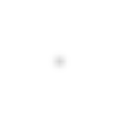
Lpoly(Kd,4,Kd,2,Ku,α,β)=∑ϕ∥F(Kd,4,Kd,2,Ku,α,β)(δϕ)−SϕGσ∥22=∑ϕ∥Rϕ−Gσ∥22.\begin{aligned} \mathcal L_{\mathrm{poly}}(K_{d,4},K_{d,2},K_u,\boldsymbol\alpha,\beta) &=\sum_{\boldsymbol\phi} \left\|\mathcal F_{(K_{d,4},K_{d,2},K_u,\boldsymbol\alpha,\beta)}(\delta_{\boldsymbol\phi}) -\mathcal S_{\boldsymbol\phi}G_\sigma\right\|_2^2 \\ &=\sum_{\boldsymbol\phi} \left\|R_{\boldsymbol\phi}-G_\sigma\right\|_2^2. \end{aligned}

Sϕ\mathcal S_{\boldsymbol\phi} translates the centered target kernel to n0+ϕ\mathbf n_0+\boldsymbol\phi. The right-hand side instead uses coordinates relative to each input point. The target moves with the input, while phase-dependent shape differences remain in the residuals.

Reevaluating all phases gives

RMSE⁡all=1P2M2∑ϕ∥Rϕ−Gσ∥22,\operatorname{RMSE}_{\mathrm{all}} =\sqrt{\frac{1}{P^2M^2} \sum_{\boldsymbol\phi}\left\|R_{\boldsymbol\phi}-G_\sigma\right\|_2^2},

where MM is the side length of one response image. The σ=4\sigma=4 experiment in this section uses M=128M=128. Worst-phase RMSE is the largest per-phase RMSE. All-phase RMSE aggregates squared errors before taking the square root; it is not the arithmetic mean of the per-phase RMSE values.

Single-phase RMSE evaluates only the directly supervised location, whereas all-phase RMSE aggregates all 64 input phases. They are not interchangeable; numerical values appear in the error table below.

2. Polyphase Optimization at a Single σ

Keeping the Same Optimization Variables

Call the polyphase optimized method C. It retains B's three ring kernels, all blend factors, nonnegative unit-sum weights, radius bounds, and cross-level sharing. It also uses the same four initializations and L-BFGS-B solver. Only the supervised set changes: B uses (0,0)(0,0), while C uses all phases.

Minimizing the Polyphase Loss

Minimizing the loss gives the polyphase optimized method C:

(Kd,4,Kd,2,Ku,α,β)C≈arg min⁡Kd,4,Kd,2,Ku,α,β  Lpoly(Kd,4,Kd,2,Ku,α,β).(K_{d,4},K_{d,2},K_u,\boldsymbol\alpha,\beta)_C\approx\underset{K_{d,4},K_{d,2},K_u,\boldsymbol\alpha,\beta}{\operatorname{arg\,min}}\; \mathcal L_{\mathrm{poly}}(K_{d,4},K_{d,2},K_u,\boldsymbol\alpha,\beta).

Computing Gradients of Weights and Sampling Offsets

Bilinear interpolation is piecewise differentiable with respect to sample positions, and a weighted sum is differentiable with respect to its weights. Both the single-phase and polyphase least-squares objectives can therefore propagate gradients through the complete chain. The first part uses the same gradient-based approach; this section adds input phases to the loss.

Updating Parameters and Comparing Results

At a fixed σ=4\sigma=4, compare the impulse and sinc outputs of Gaussian, single-phase B, and polyphase C. B and C each contain one Kd,4K_{d,4}, one Kd,2K_{d,2}, a cross-level shared KuK_u, and per-level blend factors. At runtime, the same chain processes the entire image. Complete parameter tables for each scale are in Appendix D.

σ=4 · Input phase (0,0) · Shared display gain 20×, no clipping. A—A marks the center row; the overlaid curve below shows its raw values, with Gaussian as a gray dashed reference.
Gaussian
2D RMSE 0
Gaussian full phase-zero impulse response, shared display gain 20×AA06.7e-31.3e-2-24024
A—A · Position relative to input / px
B · Single-impulse fit
2D RMSE 3.803e-5
B · Single-impulse fit full phase-zero impulse response, shared display gain 20×AA06.7e-31.3e-2-24024
A—A · Position relative to input / px
C · Polyphase optimization
2D RMSE 1.956e-4
C · Polyphase optimization full phase-zero impulse response, shared display gain 20×AA06.7e-31.3e-2-24024
A—A · Position relative to input / px

σ=4 · B/C: initial 4× downsample, 1 levels of 2× down/up · Outputs at 1×

Gaussian
Image RMSE 0
σ=4, Gaussian actual sinc-image output
B · Single-impulse fit
Image RMSE 3.486e-2
σ=4, B · Single-impulse fit actual sinc-image output
C · Polyphase optimization
Image RMSE 1.531e-2
σ=4, C · Polyphase optimization actual sinc-image output
Gaussian · AE ×1
max 0 · No clipping
σ=4, Gaussian absolute error relative to Gaussian, amplified 1×; white is zero error
B · AE ×1
max 3.066e-1 · No clipping
σ=4, B · Single-impulse fit absolute error relative to Gaussian, amplified 1×; white is zero error
C · AE ×1
max 2.209e-1 · No clipping
σ=4, C · Polyphase optimization absolute error relative to Gaussian, amplified 1×; white is zero error
Method (σ=4)Phase (0,0) RMSEAll-phase RMSEWorst-phase RMSESinc-image RMSE
B: Single-phase optimization3.803e-055.795e-048.595e-043.486e-02
C: Polyphase optimization1.956e-042.357e-043.117e-041.531e-02

At this scale, all-phase RMSE decreases by approximately 59.34%, and sinc-image RMSE by approximately 56.07%. These metrics evaluate the full impulse-response family and this particular test image, respectively.

C has a larger error than B at (0,0)(0,0), but a lower total squared error across all phases. Thus, B's single-location fit still leaves room for improvement: the same parameter family and sampling budget can produce another set of kernels and blend factors that better approximates Gaussian responses across all phases. C is still constrained by the finite sampling stencils, however, and does not guarantee identical responses at every phase.

3. Polyphase Optimization Across Multiple σ Values

Solving Each σ Independently

Each target scale requires its own level count and kernel parameters. The table below retains two independently solved scales. They establish results only for those two targets, not a continuous mapping from σ to parameters.

Target σ2× downsampling levels N (after the initial 4×)Per-axis phase period2D phase count
41864
403321024

Fitting Parameters as Functions of σ

Rerunning the Complete Chain with Fitted Parameters

Polyphase Optimization of Downsampled Blur

1. A Downsampled Blur Chain with Fixed Mipmaps

This section applies polyphase supervision to a shared mipmap-pyramid blur method: first build a shared mipmap pyramid with fixed box kernels, then use a small kernel to sample a selected mip level for each final-resolution output pixel. Blur coverage comes from the combination of the mip level and the final sampling kernel.

This method samples the mipmap directly at the final resolution, rather than following Kawase's level-by-level upsampling chain. The constraints and solution procedure are outlined below; optimization results are not yet included.

2. Optimization Variables and Runtime Constraints

  • Fixed, shared mipmap kernels. All σ values use the same fixed downsampling results. Only the final sampling weights and offsets are solved for each σ.
  • Fixed sampling budget. Specify the sample count of the final pass and use the same budget for the original and optimized methods. Record the shared mipmap construction cost separately.
  • Continuous blur radius. After parameter fitting, inspect outputs at neighboring σ values and around mip-level transitions.
  • Retain the original mip-level selection rule. Level selection is not a variable in this round of continuous parameter optimization.

3. Polyphase Optimization Across Multiple σ Values

Solving Each σ Independently

With the shared mipmap and the level for that σ fixed, enumerate input phases and build a polyphase squared-error objective for the final sampling parameters.

Fitting the Final Sampling Parameters

Rerunning the Complete Chain with Fitted Parameters

4. Comparing the Original and Polyphase Optimized Methods

Appendix: Derivations, Additional Comparisons, and Reproduction

A. Revisions to the Android Baseline

A, B, C, and the interactive demos use the same Android-derived implementation. It retains V2's initial 4× scaling, subsequent 2× scaling, inter-level blending, and original-image blending, with the following two revisions. These describe the version used in this article; they do not imply that AOSP has incorporated the changes.
Two Signs in the Direction Constants

The pinned AOSP revision describes the upsampling directions as a regular heptagon, but the signs of STEP_4.x and STEP_6.x do not match the corresponding vertices:

ConstantOriginal valueValue used here
STEP_4.x+0.900968868−0.900968868
STEP_6.x−0.623489802+0.623489802

A retains the decimal precision of those constants. B/C and the interactive demo generate directions with the trigonometric functions of a regular heptagon. The heptagon's sample positions have a zero centroid, but are not symmetric about both the x and y axes. Nor does this guarantee that the discrete response's peak lies at its centroid.

Reference-Coordinate Compensation for Downsampling and Upsampling

This article uses input phase (0,0)(0,0) as its registration reference. With integer pixel indices, the original implementation's first 4× downsample is equivalent to averaging nonoverlapping 4×44\times4 input blocks. An impulse at (256,256)(256,256) falls into the block indexed 256∼259256\sim259, corresponding to low-resolution pixel (64,64)(64,64). The original 4× reconstruction maps its center back to (257.5,257.5)(257.5,257.5), adding a displacement of 1.51.5 original-image pixels per axis to the blurred branch.

Compensation must be applied inside the sampling coordinates of every upsampling pass, before blending with a saved same-level image or the original image. For the current kernel parameters, first generate the downsampling pyramid from a fixed phase-(0,0)(0,0) impulse. Let μi\boldsymbol\mu_i be the centroid of level ii relative to its reference position, measured in that level's texels. Uncompensated 2× reconstruction maps the child centroid to 2μi+1+1212\boldsymbol\mu_{i+1}+\tfrac12\mathbf1, so the output displacement to subtract is

di=2μi+1+121−μi,oi=di/2.\mathbf d_i=2\boldsymbol\mu_{i+1}+\tfrac12\mathbf1-\boldsymbol\mu_i, \qquad \mathbf o_i=\mathbf d_i/2.

oi\mathbf o_i is the offset, in input texels, added to that pass's sampling coordinates. It gives the reconstructed branch the same reference centroid as the saved level-ii image; only then are they blended. The final 4× reconstruction uses of=μ0+381\mathbf o_f=\boldsymbol\mu_0+\tfrac38\mathbf1, returning the blurred branch to the original-image reference position before the final blend.

These offsets are determined by the kernel parameters and the fixed reference impulse; they are not extra optimization variables. One parameter set uses the same offsets for the entire image and every phase, without repositioning based on the image being processed. Optimization also propagates the offsets' derivatives with respect to the kernel parameters. A zero reference response has no centroid, so a finite neutral fallback is used while retaining the zero response and its loss.

For A's original stencils, μ0=0\boldsymbol\mu_0=0. The 2× downsampling weights give exactly di=0\mathbf d_i=0, and the final 4× reconstruction requires an output correction of 1.51.5 pixels per axis. The original and article sampling positions are then

cnative(n)=n+1/24−12,carticle(n)=cnative(n)+1.54=n4.c_{\mathrm{native}}(n)=\frac{n+1/2}{4}-\frac12, \qquad c_{\mathrm{article}}(n)=c_{\mathrm{native}}(n)+\frac{1.5}{4}=\frac n4.

This simplification does not extend to arbitrary optimized parameters. For example, if both Kd,2K_{d,2} and KuK_u collapse to center-only sampling, the child response lies at index 3232. Uncompensated 2× reconstruction centers it at parent index 64.564.5, whereas the saved parent response lies at 6464. That 2× upsampling pass therefore needs an extra 0.250.25 input texels per axis, correcting half a parent pixel to the left and up. Correcting only the final 4× reconstruction would still blend two internally misaligned branches first.

This procedure retains the downsampling and upsampling stencils and changes only a common coordinate offset for each group of samples. It adds neither prefiltering nor an extra image-translation pass. Once the kernel parameters are fixed, the reference probes and offsets can be precomputed; actual images run only the existing sampling and blending chain.

For blurRadius=6, the uncompensated phase-(0,0)(0,0) blurred branch is displaced by 1.51.5 pixels per axis, or 0.90.9 pixels after blending with the original image. Compensation returns both centroids to the input centroid within numerical error. This is coordinate compensation for a designated reference phase, not per-phase alignment. Other input locations within the same block still share the first-level samples. Moving the impulse diagonally to phases (1,1),(2,2),(3,3)(1,1),(2,2),(3,3) yields complete-output displacements of −0.6,−1.2,−1.8-0.6,-1.2,-1.8 pixels per axis. These genuine phase differences enter the main polyphase loss unchanged.

The original per-pass audit is saved in android-coordinate-audit.json. The article's version of A is checked with verify_aosp_kawase_v2_skia --registered. Its original stencils have zero internal offsets; in the independent Skia execution, the final blur shader's matrix translation is set to (−1.5,−1.5)(-1.5,-1.5) original-image pixels before comparison with the float64 implementation. CPU F32 validation covers all 64 phases at σ=4,8\sigma=4,8, eight distributed phases each at σ=16,40\sigma=16,40, the sinc image, and odd-sized image boundaries. Results are recorded in android-registered-skia-validation.json.
For variable kernels, test_android_kawase_core.py additionally covers center-only and general kernels at N=1,2,3N=1,2,3. It compares per-level centroids before and after blending and checks final reference registration, other-phase differences, direct rendering against frequency-domain evaluation, and full gradients including offset derivatives. The interactive demo has corresponding TypeScript checks.

B. Gaussian5x5 Single-Stage Impulse Experiment

Centered Impulse

This single-stage chain illustrates impulse evaluation: Gaussian5x5 prefiltering, 2× decimation on the even grid, a 7×77\times7 Gaussian with σ=1.5\sigma=1.5 at low resolution, and reconstruction with a triangle kernel. It isolates the decimation grid's effect on the impulse response. The main Kawase fits use a different, complete chain. Here, the processing chain is again denoted by P\mathcal P, with centered impulse response K=P(δ)K=\mathcal P(\delta).

Input
Discrete impulse δ\delta (enlarged center)
Discrete unit impulse at the center pixel, with the central region enlarged using nearest-neighbor sampling
Downsampled Rearrangement
d[k]d[\mathbf k]
Low-resolution centered impulse after Gaussian5x5 prefiltering, even-grid sampling, and rearrangement; brightness is peak-normalized
Output

Gaussian5x5 single-stage equivalent kernel K=P(δ)K=\mathcal P(\delta)

Output weight distribution of a centered single-pixel impulse through the single-stage Gaussian5x5 downsampling chain
Cross-Section
Center-row cross-section of equivalent kernel KK
Center-row cross-section of the equivalent convolution kernelThe horizontal axis is the original-image pixel offset from the unshifted impulse center. The vertical axis is the raw weight after a single-pixel impulse passes through the single-stage Gaussian5x5 downsampling chain.00.511.52K[x] · 10⁻²-32-1601631

Impulse Shifted One Pixel to the Right

Keep the chain and kernel parameters fixed, and move only the input impulse one pixel to the right. If the system is shift-invariant, the new output must be exactly the original response shifted right:

P(δ(x−1))=K(x−1),K=P(δ).\mathcal P\bigl(\delta(x-1)\bigr)=K(x-1), \qquad K=\mathcal P(\delta).

Using the same Gaussian5x5 single-stage demo chain and changing only the input position gives:

Input
Discrete impulse δ(x−1)\delta(x-1) (enlarged center)
Discrete unit impulse one pixel right of center, with the central region enlarged using nearest-neighbor sampling
Downsampled Rearrangement
d[k]d[\mathbf k]
Low-resolution shifted impulse after Gaussian5x5 prefiltering, even-grid sampling, and rearrangement; brightness is peak-normalized
Output

Gaussian5x5 single-stage equivalent kernel K1=P(δ(x−1))K_1=\mathcal P(\delta(x-1))

Output weight distribution of a single-pixel impulse shifted one pixel right through the same Gaussian5x5 downsampling chain
Cross-Section
Center-row cross-section of equivalent kernel K1K_1
Center-row cross-section of the shifted impulse responseThe horizontal axis is the original-image pixel offset from the unshifted impulse center. The vertical axis is the raw weight after a single-pixel impulse shifted one pixel right passes through the same chain.00.511.52K[x] · 10⁻²-32-1601631

Compared with the centered response, the output changes shape as well as position:

P(δ(x−1))≠K(x−1).\mathcal P\bigl(\delta(x-1)\bigr)\neq K(x-1).

The decimation grid remains fixed. An impulse at an even location and one at an odd location place prefiltered weights on different sample positions, changing the values that enter the low-resolution image. Reconstruction then spreads those samples back to high resolution. The input's position relative to this fixed grid is its phase.

C. Per-Phase Response Statistics

Gaussian responses are identical across phases; Kawase-chain responses can still vary with phase. A, B, and C all use period P=4⋅2NP=4\cdot2^N, giving 64 phases at σ=4\sigma=4 and 1024 at σ=40\sigma=40. The metrics enumerate every phase.

Response mass is the sum of the weights. Centroid displacement uses the input point as the origin, and per-axis σ\sigma is calculated from the second moment about the response's own centroid. Equal mass and centroid do not imply equal width, peak, or shape. The upsampling kernel is a heptagon, so responses must not be additionally averaged with their reflections about both axes. The mean-response width used for radius calibration also differs from the range of single-phase widths.

σ=4 · Each method enumerates its full period. Per-phase σ is measured about its own centroid. Zero responses have no centroid or σ and are excluded from those ranges.
MethodPhase countZero responsesResponse mass rangeNonzero per-axis σ rangeMax per-axis centroid displacement / px
Gaussian6401.000000 – 1.0000004.0000 – 4.00000.0000
Android Kawase V26401.000000 – 1.0000003.7924 – 4.11151.8000
B · Single-impulse fit6400.011936 – 1.5161973.9149 – 4.00197.9551
σ=40 · Each method enumerates its full period. Per-phase σ is measured about its own centroid. Zero responses have no centroid or σ and are excluded from those ranges.
MethodPhase countZero responsesResponse mass rangeNonzero per-axis σ rangeMax per-axis centroid displacement / px
Gaussian102401.000000 – 1.00000039.9997 – 39.99970.0000
Android Kawase V2102401.000000 – 1.00000039.6610 – 40.00733.0000
B · Single-impulse fit102400.987726 – 1.01821338.9098 – 40.79093.8414

D. Complete Parameters, Additional Comparisons, and Error Analysis

Kernel Parameters and Fit Metrics at Two Target Scales

A uses the Kawase baseline parameters described above. B and C are solved with single-phase and polyphase objectives, respectively. The tables below summarize parameters and impulse errors at σ=4\sigma=4 and σ=40\sigma=40. Each scale uses its own parameters; B and C share the same sampling budget and parameter bounds.

σ=4 · N=1
MethodKernelθ / radw_ca / input texels
B · Single-impulse fitK_d,40.5352650.3694281.752996
B · Single-impulse fitK_d,22.0132960.9999630.398384
B · Single-impulse fitK_u0.4961140.0264070.250000
C · Polyphase optimizationK_d,40.7853980.0000091.404174
C · Polyphase optimizationK_d,20.7853980.1991841.335039
C · Polyphase optimizationK_u0.1613561.0000000.250000
Methodα_0β
B · Single-impulse fit0.9887701.000000
C · Polyphase optimization0.9149170.996897
σ=40 · N=3
MethodKernelθ / radw_ca / input texels
B · Single-impulse fitK_d,40.7853980.0029481.410899
B · Single-impulse fitK_d,20.7696320.2977051.503566
B · Single-impulse fitK_u-0.1136380.3891941.573893
C · Polyphase optimizationK_d,40.7853980.0000001.414104
C · Polyphase optimizationK_d,20.7838560.0192301.140882
C · Polyphase optimizationK_u0.0043920.3733701.546569
Methodα_0α_1α_2β
B · Single-impulse fit0.9999950.9998461.0000001.000000
C · Polyphase optimization1.0000001.0000001.0000001.000000
σ=4 · Each response is 128×128 · A covers 64 phases; B/C cover 64. Each metric averages squared errors before taking the square root.
Method(0,0) RMSEAll-phase RMSEWorst-phase RMSE
Gaussian000
Android Kawase V23.262e-33.159e-33.262e-3
B · Single-impulse fit3.803e-55.795e-48.595e-4
C · Polyphase optimization1.956e-42.357e-43.117e-4
σ=40 · Each response is 512×512 · A covers 1024 phases; B/C cover 1024. Each metric averages squared errors before taking the square root.
Method(0,0) RMSEAll-phase RMSEWorst-phase RMSE
Gaussian000
Android Kawase V21.760e-61.864e-62.049e-6
B · Single-impulse fit2.063e-78.268e-71.399e-6
C · Polyphase optimization3.026e-75.494e-71.027e-6

σ=4: phase-(0,0) RMSE is 3.803e-5 for B and 1.956e-4 for C. All-phase RMSE changes from 5.795e-4 (B) to 2.357e-4 (C), a 59.34% reduction.

σ=40: phase-(0,0) RMSE is 2.063e-7 for B and 3.026e-7 for C. All-phase RMSE changes from 8.268e-7 (B) to 5.494e-7 (C), a 33.55% reduction.

Additional Sinc-Image Comparisons

First, compare Gaussian, Kawase baseline A, and single-phase B at σ=4\sigma=4; then compare Gaussian, B, and C at σ=40\sigma=40. Image computation and AE display conventions are given in Appendix E.

σ=4 · A: Android blurRadius=6; B: initial 4× downsample, 1 levels of 2× down/up · Outputs at 1×
Gaussian
Image RMSE 0
σ=4, Gaussian actual sinc-image output
Android Kawase V2
Image RMSE 5.722e-2
σ=4, Android Kawase V2 actual sinc-image output
B · Single-impulse fit
Image RMSE 3.486e-2
σ=4, B · Single-impulse fit actual sinc-image output
Gaussian · AE ×1
max 0 · No clipping
σ=4, Gaussian absolute error relative to Gaussian, amplified 1×; white is zero error
A · AE ×1
max 4.984e-1 · No clipping
σ=4, Android Kawase V2 absolute error relative to Gaussian, amplified 1×; white is zero error
B · AE ×1
max 3.066e-1 · No clipping
σ=4, B · Single-impulse fit absolute error relative to Gaussian, amplified 1×; white is zero error

σ=40 · B/C: initial 4× downsample, 3 levels of 2× down/up · Outputs at 1×

Gaussian
Image RMSE 0
σ=40, Gaussian actual sinc-image output
B · Single-impulse fit
Image RMSE 4.631e-3
σ=40, B · Single-impulse fit actual sinc-image output
C · Polyphase optimization
Image RMSE 4.596e-3
σ=40, C · Polyphase optimization actual sinc-image output
Gaussian · AE ×20
max 0 · No clipping
σ=40, Gaussian absolute error relative to Gaussian, amplified 20×; white is zero error
B · AE ×20
max 3.029e-2 · No clipping
σ=40, B · Single-impulse fit absolute error relative to Gaussian, amplified 20×; white is zero error
C · AE ×20
max 3.055e-2 · No clipping
σ=40, C · Polyphase optimization absolute error relative to Gaussian, amplified 20×; white is zero error

σ=4: sinc-image RMSE is 3.486e-2 for B and 1.531e-2 for C, a 56.07% decrease. This percentage compares only B/C, with identical sampling budgets, parameter families, and boundary rules.

σ=40: sinc-image RMSE is 4.631e-3 for B and 4.596e-3 for C, a 0.75% decrease. This percentage compares only B/C, with identical sampling budgets, parameter families, and boundary rules.

The tables report all-phase impulse errors and sinc-image errors separately. All-phase supervision improves the response objective over the full kernel support. Finite images also involve per-level clamp boundaries and the structure of the particular input. These two metrics are not interchangeable.

Mean-Kernel Shape Error and Phase Variation

To distinguish mean-shape approximation error from phase variation, take the mean of the input-aligned responses:

Rˉ=1P2∑ϕRϕ.\bar R=\frac1{P^2}\sum_{\boldsymbol\phi}R_{\boldsymbol\phi}.

The squared error has the exact decomposition

1P2∑ϕ∥Rϕ−Gσ∥22⏟Total error=∥Rˉ−Gσ∥22⏟Mean-kernel shape error+1P2∑ϕ∥Rϕ−Rˉ∥22⏟Phase variation.\underbrace{\frac1{P^2}\sum_{\boldsymbol\phi}\|R_{\boldsymbol\phi}-G_\sigma\|_2^2}_{\text{Total error}} = \underbrace{\|\bar R-G_\sigma\|_2^2}_{\text{Mean-kernel shape error}} + \underbrace{\frac1{P^2}\sum_{\boldsymbol\phi}\|R_{\boldsymbol\phi}-\bar R\|_2^2}_{\text{Phase variation}}.

The cross term vanishes because ∑ϕ(Rϕ−Rˉ)=0\sum_{\boldsymbol\phi}(R_{\boldsymbol\phi}-\bar R)=0. Even if the mean response closely matches a Gaussian, the total error remains nonzero while the phases differ. The last two table columns divide these two terms by the response pixel count and take their square roots. The sum of their squares therefore equals the square of the all-phase RMSE.

σ=4 · Sinc image: 512×512. “Interior” excludes a 32 px border. The sum of squares of the last two columns equals the all-phase RMSE squared.
MethodImage RMSEMax AEInterior RMSEMean-kernel shape RMSEPhase variation RMS
Gaussian0004.838e-190
Android Kawase V25.722e-24.984e-15.966e-23.145e-32.986e-4
B · Single-impulse fit3.486e-23.066e-13.633e-23.870e-44.314e-4
C · Polyphase optimization1.531e-22.209e-11.604e-22.000e-41.247e-4
σ=40 · Sinc image: 512×512. “Interior” excludes a 32 px border. The sum of squares of the last two columns equals the all-phase RMSE squared.
MethodImage RMSEMax AEInterior RMSEMean-kernel shape RMSEPhase variation RMS
Gaussian0001.925e-190
Android Kawase V24.809e-32.889e-22.187e-31.817e-64.121e-7
B · Single-impulse fit4.631e-33.029e-21.826e-34.441e-76.974e-7
C · Polyphase optimization4.596e-33.055e-21.713e-32.874e-74.682e-7

“Interior RMSE” excludes a 32-pixel border on all four sides of the original image. For the large-support σ=40\sigma=40 kernel, that region may still be affected by boundaries; it is not a fully boundary-free experiment.

B's single-impulse objective constrains one designated response; moving from B to C fills in the missing phase supervision. A, B, and C use the same chain structure. A only matches an integer radius, whereas B/C optimize kernel and blend parameters. The polyphase loss does not separately guarantee reductions in centroid error, worst-phase error, or error on every image.

Impulse Metrics and Actual Image Error

For input noise with independent, zero-mean, equal-variance pixels, expected output-error energy is proportional to the summed squared response errors. Real images have spatial correlations, so response errors from different locations can cancel or reinforce one another. Downsampled blur should therefore be evaluated using both the complete polyphase impulse responses and actual images: the former measures approximation across input locations; the latter tests the result for specific images and boundary conditions.

E. Numerical Configuration and Reproduction

Matching the Android Radius to the Target σ

A uses the baseline defined in Appendix A. Its stencil weights, level schedule, sampling distances, and blend factors are determined by integer blurRadius. This radius is not the Gaussian standard deviation, and the width at one phase cannot represent the whole chain.

For every candidate radius rr, align all P(r)2P(r)^2 responses in its full period to their respective input locations and average them, producing unit-mass Rˉr\bar R_r. Let its centroid be μr\boldsymbol\mu_r. The matching scale is the mean of the two central variances:

σA2(r)=12∑x∥x−μr∥22Rˉr[x],rA=arg⁡min⁡r∈Z≥0  ∣σA(r)−σ∣.\sigma_A^2(r)=\frac12\sum_{\mathbf x}\|\mathbf x-\boldsymbol\mu_r\|_2^2\bar R_r[\mathbf x],\qquad r_A=\underset{r\in\mathbb Z_{\ge0}}{\arg\min}\;|\sigma_A(r)-\sigma|.

This step matches spread only; it does not fit weights or offsets using Gaussian response-shape error. The numerical implementation propagates moments through every sample and interpolation, and is verified by explicitly enumerating all phases. It includes the initial downsample, progressive reconstruction, inter-level blending, final 4× enlargement, and small-radius blend. Measuring width with central moments does not shift the output: images and losses still use the input point as their origin.

Targets σ=4,8,16,40\sigma=4,8,16,40 select integer radii 6,17,32,906,17,32,90, with mean-response standard deviations of approximately 3.9817,8.0894,16.0737,39.85023.9817,8.0894,16.0737,39.8502. Integer steps are coarse at small radii, so width matching itself has a residual; see the table above.

To reproduce Android's internal radius schedule, the numerical port follows the source directly: ρ=0.57735r\rho=0.57735r, continuous depth d=min⁡(3,ρ/10)d=\min(3,\rho/10), N=⌈d⌉N=\lceil d\rceil, and αi=min⁡(1,d−i)\alpha_i=\min(1,d-i). The source's step, denoted by ss, is uniquely determined by these quantities; radius matching searches only over rr. In shader coordinates,

s=max⁡ ⁣(0,(ρ/4)2−∑i=0N−1(2i−1αi2)2)∑i=0N−1(2iαi)2.s=\sqrt{\frac{\max\!\left(0,(\rho/4)^2-\sum_{i=0}^{N-1}(2^{i-1}\alpha_i\sqrt2)^2\right)}{\sum_{i=0}^{N-1}(2^i\alpha_i)^2}}.

When N=0N=0, set s=0s=0. In an exactly 2× upsampling pass, ss shader pixels correspond to s/2s/2 input texels.

Static figures and numerical metrics use float64 linear luminance; the interactive σ-slider images use float32 shaders. The scope of the independent Skia checks is described in Appendix A. These are neither Android-device screenshots nor performance measurements.

Impulse Responses and Solver Configuration

GσG_\sigma is centered on the input impulse. The loss sums every pixel of the full 2D response; cross-sections are only a visualization. Fitting retains raw response values without peak or mass normalization, and evaluation does not separately recenter output centroids. The Gaussian target is truncated at 5σ5\sigma per axis and normalized. The fixed-parameter B/C comparisons use N=1N=1 with 128×128128\times128 response canvases at σ=4\sigma=4, and N=3N=3 with 512×512512\times512 canvases at σ=40\sigma=40. The final figures cover the complete kernel support. During search, if a candidate exceeds that support, the evaluation canvas expands automatically to avoid circular-convolution aliasing. Impulse rendering uses a larger zero background to isolate boundaries.

Although the residuals form a least-squares objective, the full multilevel chain depends nonlinearly on sample distances and weights. The fixed-parameter B/C comparison uses L-BFGS-B with analytic gradients and parameter bounds. It solves from four initializations for at most 180 iterations each, then retains the lowest-loss result. The solver scales the loss only by a fixed target energy, which does not change the optimum. “Optimized result” means the best result found within these bounds and initializations, not a proven global optimum.

The σ slider's 80 single-phase fits allow up to 250 iterations per initialization, with nearby-scale solutions and the same-scale single-phase parameters from Appendix D as additional starts. This parameter table is stored independently; the later all-phase statistics for B/C still correspond to the fixed parameters in Appendix D. Slider rendering and RMSE computation use 512×512512\times512, while fitting adapts the canvas to kernel support. Both contain the complete response, so the ratio of squared error to target energy is unaffected by the amount of zero background.

The large-scale chain has 1024 phases. To avoid retaining 1024 large response images during optimization, the numerical implementation uses correlation operations on the cascaded filters to compute the exact all-phase squared error and its gradient. This is equivalent to summing the objectives for every phase individually. The final kernels are also checked against an independent per-pixel sampling and blending chain, and evaluation explicitly enumerates all phases.

Image and Error Display Conventions

Each comparison identifies its participating methods in the headings. Static images are computed in float64 linear luminance. A/B/C use clamp boundaries inside the pyramid and mirror boundaries for final reconstruction; Gaussian uses clamp. In comparisons with AE, each column shows the actual output above its absolute error relative to Gaussian: AE=∣Imethod−IG∣\mathrm{AE}=|I_{\mathrm{method}}-I_G|.

All static outputs are displayed at 1×1\times. Within one scale, AE uses the fixed gain indicated in the figure, with white representing zero error and no display clipping. The two scales use different gains, so error magnitudes cannot be compared across scales by darkness alone. Gaussian's error against itself is entirely white. The σ slider's raw mode displays response hh on white as 1−h1-h; enhanced mode uses exp⁡(−2.5h/Gσ(0,0))\exp(-2.5h/G_\sigma(0,0)). Display values are clamped to [0,1][0,1]; raw curves and metrics do not use this mapping.

Reproduction Commands and Validation Scope

The four opening Gaussian / Android V2 comparisons can be generated separately with python3 -m scripts.generate_android_sinc_comparison. Radii, image errors, and the source-image hash are recorded in content/blog/differentiable-polyphase-filtering/android-sinc-comparison-data.json.

Regenerate σ-slider parameters with python3 -m scripts.fit_single_phase_sweep, which requires NumPy, SciPy, and Numba. --resume continues from saved settings, and --workers 1 uses one process. After the first round, run python3 -m scripts.fit_single_phase_sweep --polish to add neighboring same-level settings as initializations. single-phase-sweep-data.json stores each setting's parameters, coordinate compensation, integer radius, initializations, and final losses. Then run bun scripts/generate_single_phase_cache.ts to package shader parameters, float64 cross-sections, and errors into one compressed cache, without storing images for every setting. python3 -m unittest scripts.test_single_phase_sweep checks full spatial rendering, frequency-domain loss, and gradients. bun test content/blog/differentiable-polyphase-filtering/single-phase-response.test.ts checks all 80 reference responses, zero-scale passthrough, and agreement between the cache, source parameters, center-row samples, and errors. single-phase-image.test.ts separately checks software mirror extension, Gaussian agreement with direct 2D convolution, and preservation of the existing impulse responses and constant inputs under mirror boundaries.

Reproduction. Running python3 -m scripts.fit_polyphase_dual_kawase solves B/C again and generates the figures and content/blog/differentiable-polyphase-filtering/four-way-blur-data.json. Add --reuse-fits to regenerate results directly from saved parameters. The data records the source-image hash, sampling conventions, final positions and weights, all-phase metrics, and losses from the four initializations. The optimizable full chain is in scripts/android_kawase_core.py; the Android V2 port and radius calibration are in scripts/aosp_kawase_v2.py. Validate with python3 -m unittest scripts.test_android_kawase_core scripts.test_polyphase_dual_kawase scripts.test_aosp_kawase_v2 scripts.test_aosp_kawase, covering per-pass sampling, analytic gradients, all-phase loss, an independent renderer, and image metrics.

Optionally install skia-python==144.0.post2 and run python3 -m scripts.verify_aosp_kawase_v2_skia --registered --sigmas 4 8 16 40 to check the article baseline. Omitting --registered checks the historical version in scripts/aosp_kawase_v2_reference.py, which changes only the two signs. Validation records for both versions and an explanation of their position differences are in Appendix A.

F. Legacy Android Kawase Reference

AOSP also includes the older KawaseBlurFilter.cpp. Its initial 4× downsample already uses radius-dependent offsets. It then runs up to four blur passes at the same low resolution, each sampling the center and four diagonals with weight 1/51/5 per tap. Its sampling coverage and pyramid structure differ from the V2 implementation used for A.

Matching the legacy implementation to σ=40\sigma=40 using the same mean-response width criterion selects blurRadius=92. Its first pass has an original-image offset of 11.511.5 and sampling centers at 4k+1.54k+1.5. It reads only input pixels whose per-axis indices are congruent to one or two modulo four, completely missing impulses in 12 of the 16 phases. The original V2 implementation covers the complete initial 4×44\times4 block, avoiding these complete omissions; the main article uses the coordinate convention defined in Appendix A. The legacy numerical port and validation are retained in scripts/aosp_kawase.py and scripts/test_aosp_kawase.py, and are not included in A's data.